在我读研时,导师的项目是做一个无人水质检测船。其目标之一是具备绘制水域的深度图的功能。基本流程是在调查水域时用无人船载着一个深度计记录水域各处的位置和深度${ \left( x,y,z \right) }$,然后根据测得的数据用LabView渲染成一个水域深度3D图。因为无人船测量深度数据的位置${ \left( x,y \right) }$是随机的,而LabView渲染3D数据需要数据按照网格排列(即二维数组的行与行、列与列之间是等距的),所以需要对无人船测量数据进行插值处理后再渲染。当时我采用的是基于径向基函数的拟合方法将随机数据插值成网格数据,效果不太好,因为径向基函数往往会在数据稀疏的地方形成一个凸起的轮廓。
偶然再次想起这个问题,虽然现在的我已不需要做这些事,但是解决这个问题可以使能力得到一些提升。经过查找,发现可以先用Delaunay三角剖分算法将测量数据拆分成一个个相邻的三角形,然后用三点线性插值法将数据修改成按网格排列的深度数据。这里不赘述理论,直接给出实现代码和效果。为了实现上的方便,本文的插值方法使用OpenCV实现,因为OpenCV已经封装好Delaunay三角剖分算法了;而3D曲面渲染使用LabView实现。OpenCV是64位的,LabView是32位的,二者通过控制台标准输入输出流共享数据。本文的运行环境是VS2017、OpenCV430和LabView2018(32位)。下面是CPP文件内容,实现了插值算法:
template<typename T1, typename T2>
float distance(const T1& p1, const T2& p2)
{
    return sqrtf((p1.x - p2.x) * (p1.x - p2.x) + (p1.y - p2.y) * (p1.y - p2.y));
}

float interpolate(const Point3f& p1, const Point3f& p2, const Point3f& p3, const Point2f& pt)
{
    float d1 = 0.5f * (distance(p1, p2) + distance(p1, pt) + distance(p2, pt));
    float s1 = sqrtf(d1 * (d1 - distance(p1, p2)) * (d1 - distance(p1, pt)) * (d1 - distance(p2, pt)));
    float d2 = 0.5f * (distance(p1, p3) + distance(p1, pt) + distance(p3, pt));
    float s2 = sqrtf(d2 * (d2 - distance(p1, p3)) * (d2 - distance(p1, pt)) * (d2 - distance(p3, pt)));
    float d3 = 0.5f * (distance(p2, p3) + distance(p2, pt) + distance(p3, pt));
    float s3 = sqrtf(d3 * (d3 - distance(p2, p3)) * (d3 - distance(p2, pt)) * (d3 - distance(p3, pt)));
    float ssum = s1 + s2 + s3;
    float z = (s1 * p3.z + s2 * p2.z + s3 * p1.z) / ssum;
    return z;
}

void interpolate(const Point3f* points, int count, const Size& size, float* xs, float* ys, float* zs)
{
    vector<Point2f> xys;
    xys.reserve(count);
    for (int i = 0; i < count; i++)
    {
        xys.push_back(Point2f(points[i].x, points[i].y));
    }
    Rect rect = boundingRect(xys);
    Subdiv2D div(rect);
    for (int i = 0; i < count; i++)
    {
        div.insert(xys);
    }
    vector<Vec6f> tris;
    div.getTriangleList(tris);
    float hStep = rect.height / (size.height - 1.0f);
    float wStep = rect.width / (size.width - 1.0f);
    for (int i = 0; i < size.height; i++)
    {
        Point2f curr;
        curr.x = rect.x + i * hStep;
        xs[i] = curr.x;
        for (int j = 0; j < size.width; j++)
        {
            curr.y = rect.y + j * wStep;
            ys[j] = curr.y;
            auto found = std::find_if(tris.begin(), tris.end(),
                [&curr](Vec6f& pt3) { return pointPolygonTest(Mat(3, 1, CV_32FC2, pt3.val), curr, false) >= 0; });
            if (found != tris.end())
            {
                auto p1 = std::find_if(points, points + count,
                    [&found](const Point3f& p) { return p.x == (*found)[0] && p.y == (*found)[1]; });
                auto p2 = std::find_if(points, points + count,
                    [&found](const Point3f& p) { return p.x == (*found)[2] && p.y == (*found)[3]; });
                auto p3 = std::find_if(points, points + count,
                    [&found](const Point3f& p) { return p.x == (*found)[4] && p.y == (*found)[5]; });
                *zs = interpolate(*p1, *p2, *p3, curr);
            }
            else
            {
                *zs = 0;
            }
            zs++;
        }
    }
}

int main()
{
    int count;
    std::cin >> count;
    std::vector<Point3f> input;
    for (int i = 0; i < count; i++)
    {
        Point3f temp;
        std::cin >> temp.x >> temp.y >> temp.z;
        input.push_back(temp);
    }
    Size size;
    std::cin >> size.width >> size.height;

    std::vector<float> xs(size.height), ys(size.width);
    std::vector<float> zs(size.area());
    interpolate(input.data(), count, size, xs.data(), ys.data(), zs.data());

    for (auto& item : xs)
    {
        std::cout << item << " ";
    }
    std::cout << "\n";

    for (auto& item : ys)
    {
        std::cout << item << " ";
    }
    std::cout << "\n";

    for (auto& item : zs)
    {
        std::cout << item << " ";
    }
    std::cout << "\n";

    return 0;
}
在三角剖分之后的三点插值方法如下。图中A、B、C是已知点,O是待插值点:
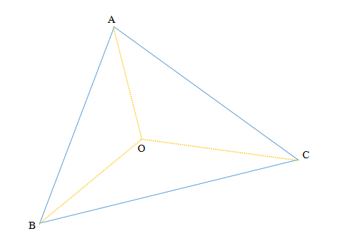
用如下公式计算O点的深度值:
$${ O_{z}=\frac{S_{\bigtriangleup OBC}}{S_{\bigtriangleup ABC}}A_{z}+\frac{S_{\bigtriangleup OAC}}{S_{\bigtriangleup ABC}}B_{z}+\frac{S_{\bigtriangleup OAB}}{S_{\bigtriangleup ABC}}C_{z} }$$
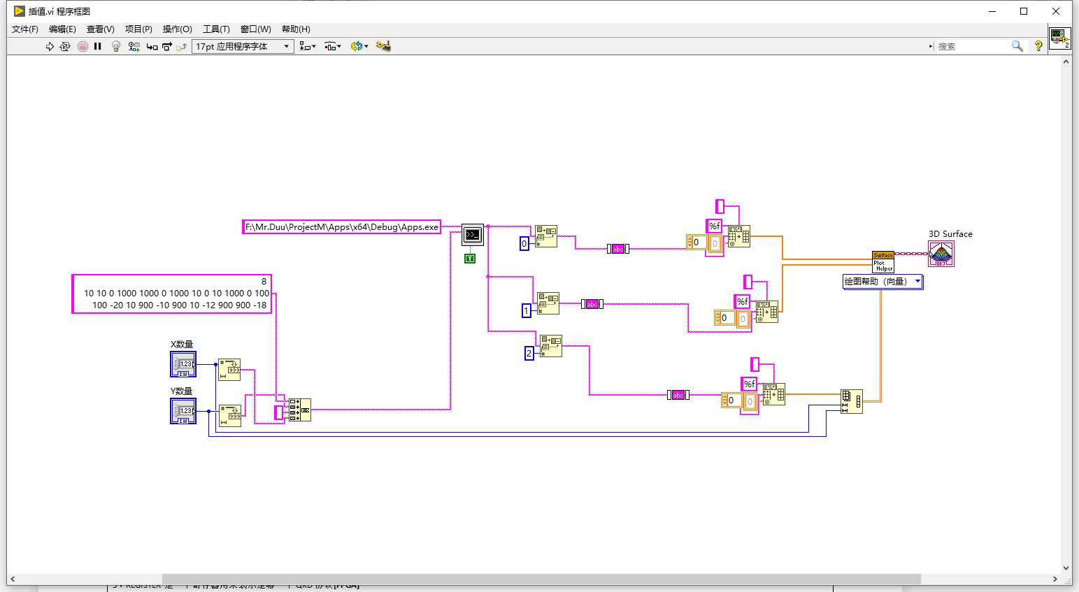
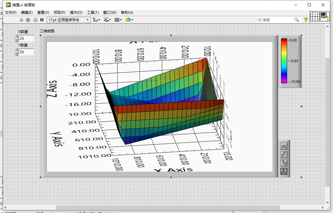
下面是LabView端的程序和界面截图。主要方法就是使用LabView的“执行系统命令”函数执行上方的C++控制台程序,把输入数据转换成字符串作为标准输入传入,程序处理之后在标准输出上打印结果,LabView读取标准输出得到结果然后显示结果。由于验证用的点比较少只有8个点,所以3D曲面看起来非常生硬: