【深度学习】总目录
- 输入端:数据增强、锚框计算等。
- backbone:进行特征提取。常用的骨干网络有VGG,ResNet,DenseNet,MobileNet,EfficientNet,CSPDarknet 53,Swin Transformer等。(其中yolov5s采用CSPDarknet 53作为骨干网)应用到不同场景时,可以对模型进行微调,使其更适用于特定的场景。
- neck:neck的设计是为了更好的利用backbone提取的特征,在不同阶段对backbone提取的特征图进行在加工和合理利用。常用的结构有FPN,PANet,NAS-FPN,BiFPN,ASFF,SFAM等。(其中yolov5采用PAN结构)共同点是反复使用各种上下采样,拼接,点和和点积来设计聚合策略。
- Head:骨干网作为一个分类网络,无法完成定位任务,Head通过骨干网提取的特征图来检测目标的位置和类别。
1 输入端
1.1 数据增强
LoadImagesAndLabels类自定义了数据集的处理过程,该类继承pytorch的Dataset类,需要实现父类的__init__方法, __getitem__方法和__len__方法, 在每个step训练的时候,DataLodar迭代器通过__getitem__方法获取一批训练数据。自定义数据集的重点是 __getitem__函数,各种数据增强的方式就是在这里进行的。
1.1.1 MixUp数据增强
论文(ICLR2018收录):mixup: BEYOND EMPIRICAL RISK MINIMIZATION
Mixup数据增强核心思想是从每个Batch中随机选择两张图片,并以一定比例混合生成新的图像,训练过程全部采用混合的新图像训练,原始图像不再参与训练。
假设图像1坐标为(xi,yi),图像2坐标为(xj,yj),混合图像坐标为(x',y'),则混合公式如下:
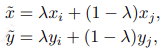
λ∈[0,1],为服从Beta分布(参数都为α)的随机数。
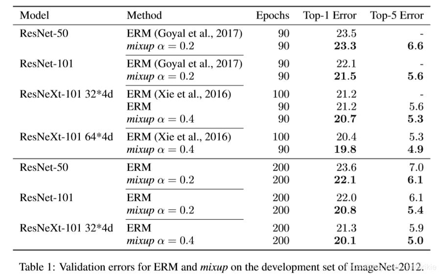
从原文实验结果中可以看出,mixup在ImageNet-2012上面经过200 epoch后在几个网络上提高了1.2 ~ 1.5个百分点。在CIFAR-10上提高1.0 ~ 1.4个百分点,在CIFAR-100上提高1.9 ~ 4.5个百分点。
Yolov5中的mixup实现
def mixup(im, labels, im2, labels2):
    # Applies MixUp augmentation https://arxiv.org/pdf/1710.09412.pdf
    r = np.random.beta(32.0, 32.0)  # mixup ratio, alpha=beta=32.0
    im = (im * r + im2 * (1 - r)).astype(np.uint8)  # 混合图像
    labels = np.concatenate((labels, labels2), 0)  # 标签直接concate更加简单
    return im, labels
1.1.2 Cutout数据增强
Cutout论文:Improved Regularization of Convolutional Neural Networks with Cutout
CNN具有非常强大的能力,然而,由于它的学习能力非常强,有时会导致过拟合现象的出现。为了解决这个问题,文章提出了一种简单的正则化方法:cutout。它的原理是在训练时随机地屏蔽输入图像中的方形区域。类似于dropout,但有两个主要的区别:(1)它丢弃的是输入图像的数据。(2)它丢弃的是一整块区域,而不是单个神经元。这能够有效地帮助CNN关注不同的特征,因为去除一个区域的神经元可以很好地防止被去除的神经元信息通过其它渠道向下传递。同时,dropout由于(1)卷积层拥有相较于全连接层更少的参数,因此正则化的效果相对欠佳;(2)图像的相邻元素有着很强的相关性的原因,在卷积层的效果不好。而cutout因为去除了一块区域的神经元,且它相比更接近于数据增强。因此在卷积层的效果要相对更好。cutout不仅容易实现,且实验证明,它能够与其它的数据增强方法一起作用,来提高模型的表现。作者发现,比起形状,cutout区域的大小更为重要。因此为了简化,他们选择了方形,且如果允许cutout区域延伸到图像外,效果反而会更好。
Yolov5中的cutout实现(默认不启用)
def cutout(im, labels, p=0.5):
    # Applies image cutout augmentation https://arxiv.org/abs/1708.04552
    if random.random() < p:
        h, w = im.shape[:2]
        scales = [0.5] * 1 + [0.25] * 2 + [0.125] * 4 + [0.0625] * 8 + [0.03125] * 16  # image size fraction
        for s in scales:
            mask_h = random.randint(1, int(h * s))  # create random masks
            mask_w = random.randint(1, int(w * s))

            # box
            xmin = max(0, random.randint(0, w) - mask_w // 2)
            ymin = max(0, random.randint(0, h) - mask_h // 2)
            xmax = min(w, xmin + mask_w)
            ymax = min(h, ymin + mask_h)

            # apply random color mask
            im[ymin:ymax, xmin:xmax] = [random.randint(64, 191) for _ in range(3)]

            # return unobscured labels
            if len(labels) and s > 0.03:
                box = np.array([xmin, ymin, xmax, ymax], dtype=np.float32)
                ioa = bbox_ioa(box, labels[:, 1:5])  # intersection over area
                labels = labels[ioa < 0.60]  # remove >60% obscured labels

    return labels
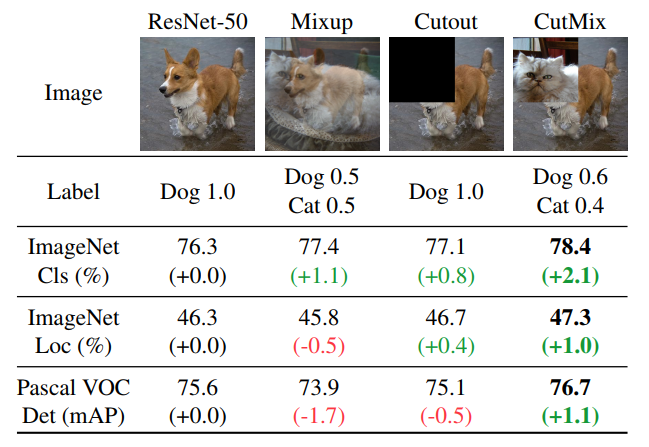
CutMix
CutMix论文:CutMix:Regularization Strategy to Train Strong Classifiers with Localizable Features
- mixup:混合后的图像在局部是模糊和不自然的,因此会混淆模型,尤其是在定位方面。
- cutout:被cutout的部分通常用0或者随机噪声填充,这就导致在训练过程中这部分的信息被浪费掉了。
cutmix在cutout的基础上进行改进,cutout的部分用另一张图像上cutout的部分进行填充,这样即保留了cutout的优点:让模型从目标的部分视图去学习目标的特征,让模型更关注那些less discriminative的部分。同时比cutout更高效,cutout的部分用另一张图像的部分进行填充,让模型同时学习两个目标的特征。
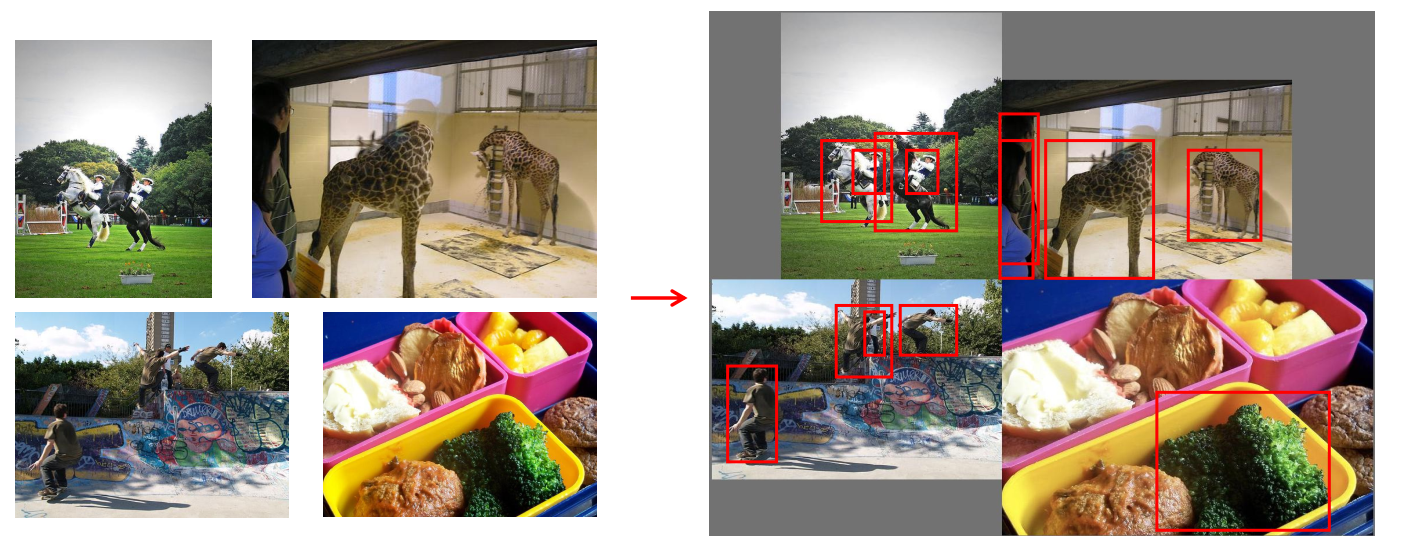
1.1.3 Mosaic数据增强
Mosaic是YOLOV4中提出的新方法,参考2019年底提出的CutMix数据增强的方式,但CutMix只使用了两张图片进行拼接,而Mosaic数据增强则采用了4张图片,通过随机缩放、随机裁减、随机排布的方式进行拼接。Mosaic有如下优点:
(1)丰富数据集:随机使用4张图片,随机缩放,再随机分布进行拼接,大大丰富了检测数据集,特别是随机缩放增加了很多小目标,让网络的鲁棒性更好;
(2)减少GPU显存:直接计算4张图片的数据,使得Mini-batch大小并不需要很大就可以达到比较好的效果。
-
初始化整个背景图, 大小为(2 × image_size, 2 × image_size, 3)
-
保留一些边缘留白,随机取一个中心点
-
基于中心点分别将4个图放到左上、右上、左下、右下,此部分可能会出现小图出界的情况,所以拼接的时候可能会进行裁剪
-
计算真实框的偏移量,在大图中重新计算框的位置
Yolov5中的4-mosaic和9-mosaic实现
    def load_mosaic(self, index):
        # YOLOv5 4-mosaic loader. Loads 1 image + 3 random images into a 4-image mosaic
        labels4, segments4 = [], []
        s = self.img_size
        yc, xc = (int(random.uniform(-x, 2 * s + x)) for x in self.mosaic_border)  # mosaic center x, y 有范围限制,左右留下mosaic_border大小边界
        indices = [index] + random.choices(self.indices, k=3)  # 在所有图片中随机选择三张
        random.shuffle(indices)
        for i, index in enumerate(indices):
            # Load image
            img, _, (h, w) = self.load_image(index)

            # place img in img4
            if i == 0:  # top left
                img4 = np.full((s * 2, s * 2, img.shape[2]), 114, dtype=np.uint8)  # base image with 4 tiles (np.full用固定值填充2s*2s的大图)
                x1a, y1a, x2a, y2a = max(xc - w, 0), max(yc - h, 0), xc, yc  # xmin, ymin, xmax, ymax (large image)
                x1b, y1b, x2b, y2b = w - (x2a - x1a), h - (y2a - y1a), w, h  # xmin, ymin, xmax, ymax (small image)
            elif i == 1:  # top right
                x1a, y1a, x2a, y2a = xc, max(yc - h, 0), min(xc + w, s * 2), yc
                x1b, y1b, x2b, y2b = 0, h - (y2a - y1a), min(w, x2a - x1a), h
            elif i == 2:  # bottom left
                x1a, y1a, x2a, y2a = max(xc - w, 0), yc, xc, min(s * 2, yc + h)
                x1b, y1b, x2b, y2b = w - (x2a - x1a), 0, w, min(y2a - y1a, h)
            elif i == 3:  # bottom right
                x1a, y1a, x2a, y2a = xc, yc, min(xc + w, s * 2), min(s * 2, yc + h)  # 在大图中每张小图的位置
                x1b, y1b, x2b, y2b = 0, 0, min(w, x2a - x1a), min(y2a - y1a, h)  # 每张小图中对应大小的区域

            img4[y1a:y2a, x1a:x2a] = img[y1b:y2b, x1b:x2b]  # img4[ymin:ymax, xmin:xmax] 将小图拷贝到大图中对应位置
            padw = x1a - x1b  # 小图的左上角点相对于大图左上角点的偏移(padw, padh),用来计算mosaic增强后的标签框的位置
            padh = y1a - y1b

            # Labels
            labels, segments = self.labels[index].copy(), self.segments[index].copy()
            if labels.size:
                labels[:, 1:] = xywhn2xyxy(labels[:, 1:], w, h, padw, padh)  # normalized xywh to pixel xyxy format
                segments = [xyn2xy(x, w, h, padw, padh) for x in segments]
            labels4.append(labels)
            segments4.extend(segments)

        # Concat/clip labels
        labels4 = np.concatenate(labels4, 0)
        for x in (labels4[:, 1:], *segments4):
            np.clip(x, 0, 2 * s, out=x)  # clip when using random_perspective()
        # img4, labels4 = replicate(img4, labels4)  # replicate

        # Augment
        img4, labels4, segments4 = copy_paste(img4, labels4, segments4, p=self.hyp['copy_paste'])
        img4, labels4 = random_perspective(img4,
                                           labels4,
                                           segments4,
                                           degrees=self.hyp['degrees'],
                                           translate=self.hyp['translate'],
                                           scale=self.hyp['scale'],
                                           shear=self.hyp['shear'],
                                           perspective=self.hyp['perspective'],
                                           border=self.mosaic_border)  # border to remove

        return img4, labels4
    def load_mosaic9(self, index):
        # YOLOv5 9-mosaic loader. Loads 1 image + 8 random images into a 9-image mosaic
        labels9, segments9 = [], []
        s = self.img_size
        indices = [index] + random.choices(self.indices, k=8)  # 8 additional image indices
        random.shuffle(indices)
        hp, wp = -1, -1  # height, width previous
        for i, index in enumerate(indices):
            # Load image
            img, _, (h, w) = self.load_image(index)

            # place img in img9
            if i == 0:  # center
                img9 = np.full((s * 3, s * 3, img.shape[2]), 114, dtype=np.uint8)  # base image with 4 tiles
                h0, w0 = h, w
                c = s, s, s + w, s + h  # xmin, ymin, xmax, ymax (base) coordinates
            elif i == 1:  # top
                c = s, s - h, s + w, s
            elif i == 2:  # top right
                c = s + wp, s - h, s + wp + w, s
            elif i == 3:  # right
                c = s + w0, s, s + w0 + w, s + h
            elif i == 4:  # bottom right
                c = s + w0, s + hp, s + w0 + w, s + hp + h
            elif i == 5:  # bottom
                c = s + w0 - w, s + h0, s + w0, s + h0 + h
            elif i == 6:  # bottom left
                c = s + w0 - wp - w, s + h0, s + w0 - wp, s + h0 + h
            elif i == 7:  # left
                c = s - w, s + h0 - h, s, s + h0
            elif i == 8:  # top left
                c = s - w, s + h0 - hp - h, s, s + h0 - hp

            padx, pady = c[:2]
            x1, y1, x2, y2 = (max(x, 0) for x in c)  # allocate coords

            # Labels
            labels, segments = self.labels[index].copy(), self.segments[index].copy()
            if labels.size:
                labels[:, 1:] = xywhn2xyxy(labels[:, 1:], w, h, padx, pady)  # normalized xywh to pixel xyxy format
                segments = [xyn2xy(x, w, h, padx, pady) for x in segments]
            labels9.append(labels)
            segments9.extend(segments)

            # Image
            img9[y1:y2, x1:x2] = img[y1 - pady:, x1 - padx:]  # img9[ymin:ymax, xmin:xmax]
            hp, wp = h, w  # height, width previous

        # Offset
        yc, xc = (int(random.uniform(0, s)) for _ in self.mosaic_border)  # mosaic center x, y
        img9 = img9[yc:yc + 2 * s, xc:xc + 2 * s]

        # Concat/clip labels
        labels9 = np.concatenate(labels9, 0)
        labels9[:, [1, 3]] -= xc
        labels9[:, [2, 4]] -= yc
        c = np.array([xc, yc])  # centers
        segments9 = [x - c for x in segments9]

        for x in (labels9[:, 1:], *segments9):
            np.clip(x, 0, 2 * s, out=x)  # clip when using random_perspective()
        # img9, labels9 = replicate(img9, labels9)  # replicate

        # Augment
        img9, labels9 = random_perspective(img9,
                                           labels9,
                                           segments9,
                                           degrees=self.hyp['degrees'],
                                           translate=self.hyp['translate'],
                                           scale=self.hyp['scale'],
                                           shear=self.hyp['shear'],
                                           perspective=self.hyp['perspective'],
                                           border=self.mosaic_border)  # border to remove

        return img9, labels9
切换使用
mosaic = self.mosaic and random.random() < hyp['mosaic']
if mosaic:
	# Load mosaic
	img, labels = load_mosaic(self, index)  # use load_mosaic4
	# img, labels = load_mosaic9(self, index)   # use load_mosaic9
	shapes = None

	# MixUp augmentation
	if random.random() < hyp['mixup']:
	    img, labels = mixup(img, labels, *load_mosaic(self, random.randint(0, self.n - 1)))
	    # img, labels = mixup(img, labels, *load_mosaic9(self, random.randint(0, self.n - 1)))
1.1.4 Copy paste数据增强
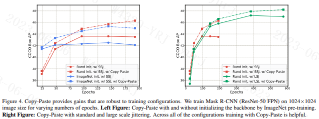
论文:Simple Copy-Paste is a Strong Data Augmentation Method for Instance Segmentation
中文名叫复制粘贴大法,将部分目标随机的粘贴到图片中,前提是数据要有segments数据才行,即每个目标的实例分割信息。
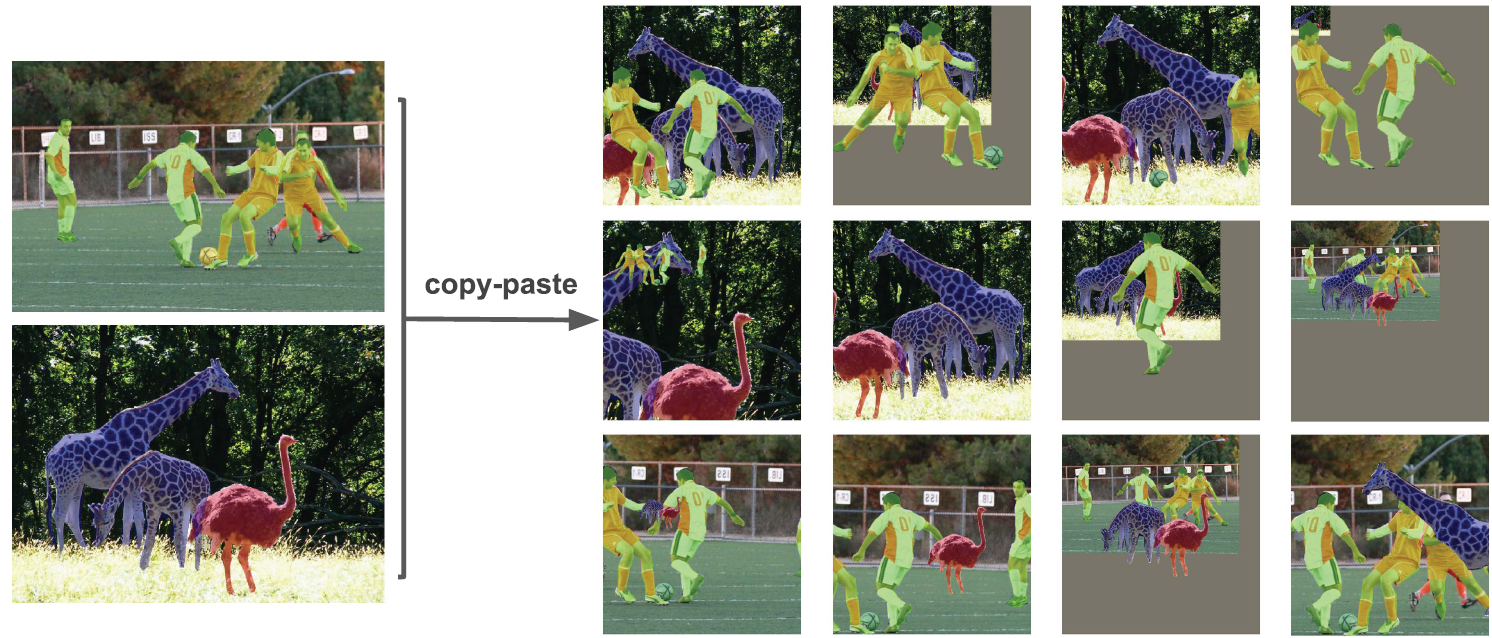
在COCO实例分割上,实现了49.1%mask AP和57.3%box AP,与之前的最新技术相比,分别提高了+0.6%mask AP和+1.5%box AP。
Yolov5中的copy paste实现
def copy_paste(im, labels, segments, p=0.5):
    # Implement Copy-Paste augmentation https://arxiv.org/abs/2012.07177, labels as nx5 np.array(cls, xyxy)
    n = len(segments)
    if p and n:
        h, w, c = im.shape  # height, width, channels
        im_new = np.zeros(im.shape, np.uint8)
        for j in random.sample(range(n), k=round(p * n)):
            l, s = labels[j], segments[j]
            box = w - l[3], l[2], w - l[1], l[4]
            ioa = bbox_ioa(box, labels[:, 1:5])  # intersection over area
            if (ioa < 0.30).all():  # allow 30% obscuration of existing labels
                labels = np.concatenate((labels, [[l[0], *box]]), 0)
                segments.append(np.concatenate((w - s[:, 0:1], s[:, 1:2]), 1))
                cv2.drawContours(im_new, [segments[j].astype(np.int32)], -1, (255, 255, 255), cv2.FILLED)

        result = cv2.bitwise_and(src1=im, src2=im_new)
        result = cv2.flip(result, 1)  # augment segments (flip left-right)
        i = result > 0  # pixels to replace
        # i[:, :] = result.max(2).reshape(h, w, 1)  # act over ch
        im[i] = result[i]  # cv2.imwrite('debug.jpg', im)  # debug

    return im, labels, segments
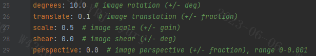
1.1.5 Random affine仿射变换
在yolov5中Mosaic数据增强部分的代码包括了仿射变换,如果部采用Mosaic数据增强也会单独进行仿射变换。yolov5的仿射变换包含随机旋转、平移、缩放、错切(将所有点沿某一指定方向成比例地平移)、透视操作,根据hyp.scratch-low.yaml,默认情况下只使用了Scale和Translation即缩放和平移。通过degrees设置图片旋转角度,perspective、shear设置透视变换和错切。
Yolov5中的random_perspective实现
def random_perspective(im,
                       targets=(),
                       segments=(),
                       degrees=10,
                       translate=.1,
                       scale=.1,
                       shear=10,
                       perspective=0.0,
                       border=(0, 0)):
    # torchvision.transforms.RandomAffine(degrees=(-10, 10), translate=(0.1, 0.1), scale=(0.9, 1.1), shear=(-10, 10))
    # targets = [cls, xyxy]

    height = im.shape[0] + border[0] * 2  # shape(h,w,c)
    width = im.shape[1] + border[1] * 2

    # Center
    C = np.eye(3)
    C[0, 2] = -im.shape[1] / 2  # x translation (pixels)
    C[1, 2] = -im.shape[0] / 2  # y translation (pixels)

    # Perspective
    P = np.eye(3)
    P[2, 0] = random.uniform(-perspective, perspective)  # x perspective (about y)
    P[2, 1] = random.uniform(-perspective, perspective)  # y perspective (about x)

    # Rotation and Scale
    R = np.eye(3)
    a = random.uniform(-degrees, degrees)
    # a += random.choice([-180, -90, 0, 90])  # add 90deg rotations to small rotations
    s = random.uniform(1 - scale, 1 + scale)
    # s = 2 ** random.uniform(-scale, scale)
    R[:2] = cv2.getRotationMatrix2D(angle=a, center=(0, 0), scale=s)

    # Shear
    S = np.eye(3)
    S[0, 1] = math.tan(random.uniform(-shear, shear) * math.pi / 180)  # x shear (deg)
    S[1, 0] = math.tan(random.uniform(-shear, shear) * math.pi / 180)  # y shear (deg)

    # Translation
    T = np.eye(3)
    T[0, 2] = random.uniform(0.5 - translate, 0.5 + translate) * width  # x translation (pixels)
    T[1, 2] = random.uniform(0.5 - translate, 0.5 + translate) * height  # y translation (pixels)

    # Combined rotation matrix
    M = T @ S @ R @ P @ C  # order of operations (right to left) is IMPORTANT
    if (border[0] != 0) or (border[1] != 0) or (M != np.eye(3)).any():  # image changed
        if perspective:
            im = cv2.warpPerspective(im, M, dsize=(width, height), borderValue=(114, 114, 114))# 透视变换
        else:  # affine
            im = cv2.warpAffine(im, M[:2], dsize=(width, height), borderValue=(114, 114, 114))# 仿射变换

    # Visualize
    # import matplotlib.pyplot as plt
    # ax = plt.subplots(1, 2, figsize=(12, 6))[1].ravel()
    # ax[0].imshow(im[:, :, ::-1])  # base
    # ax[1].imshow(im2[:, :, ::-1])  # warped

    # Transform label coordinates
    n = len(targets)
    if n:
        use_segments = any(x.any() for x in segments)
        new = np.zeros((n, 4))
        if use_segments:  # warp segments
            segments = resample_segments(segments)  # upsample
            for i, segment in enumerate(segments):
                xy = np.ones((len(segment), 3))
                xy[:, :2] = segment
                xy = xy @ M.T  # transform
                xy = xy[:, :2] / xy[:, 2:3] if perspective else xy[:, :2]  # perspective rescale or affine

                # clip
                new[i] = segment2box(xy, width, height)

        else:  # warp boxes
            xy = np.ones((n * 4, 3))
            xy[:, :2] = targets[:, [1, 2, 3, 4, 1, 4, 3, 2]].reshape(n * 4, 2)  # x1y1, x2y2, x1y2, x2y1
            xy = xy @ M.T  # transform
            xy = (xy[:, :2] / xy[:, 2:3] if perspective else xy[:, :2]).reshape(n, 8)  # perspective rescale or affine

            # create new boxes
            x = xy[:, [0, 2, 4, 6]]
            y = xy[:, [1, 3, 5, 7]]
            new = np.concatenate((x.min(1), y.min(1), x.max(1), y.max(1))).reshape(4, n).T

            # clip
            new[:, [0, 2]] = new[:, [0, 2]].clip(0, width)
            new[:, [1, 3]] = new[:, [1, 3]].clip(0, height)

        # filter candidates 对label进行面积,长宽和长宽比筛选
        i = box_candidates(box1=targets[:, 1:5].T * s, box2=new.T, area_thr=0.01 if use_segments else 0.10)
        targets = targets[i]
        targets[:, 1:5] = new[i]

    return im, targets
1.1.6 HSV随机增强图像
Yolov5使用hsv增强的目的是令模型在训练过程中看到的数据更加的多样,而通过HSV增强获得的”多样性“也可以从3个角度来说:
- 色调(Hue)多样:通过随机地调整色调可以模拟不同颜色风格的输入图像,比如不同滤镜,不同颜色光照等场景下的图像,从而提升模型在这些场景下的泛化能力;
- 饱和度(Saturation)多样:通过随机调整饱和度可以提升模型对不同鲜艳程度的目标的识别的泛化能力;
- 亮度(Value)多样:通过随机调整亮度可以提升模型应对不同光亮场景下的输入图像。
HSV增强在目标检测模型的训练中是非常常用的方法,它在不破坏图像中关键信息的前提下提高了数据集的丰富程度,且计算成本很低,是很实用的数据增强方法。
Yolov5中的augment_hsv实现
def augment_hsv(im, hgain=0.5, sgain=0.5, vgain=0.5):
    # HSV color-space augmentation
    if hgain or sgain or vgain:
        r = np.random.uniform(-1, 1, 3) * [hgain, sgain, vgain] + 1  # random gains
        hue, sat, val = cv2.split(cv2.cvtColor(im, cv2.COLOR_BGR2HSV)) #由bgr转为hsv后分离三通道
        dtype = im.dtype  # uint8
        # 创建3个通道的查找表,将通过查找表将原值映射为新值
        x = np.arange(0, 256, dtype=r.dtype)
        lut_hue = ((x * r[0]) % 180).astype(dtype)  # opencv中hue值的范围0~180
        lut_sat = np.clip(x * r[1], 0, 255).astype(dtype)
        lut_val = np.clip(x * r[2], 0, 255).astype(dtype)
        # H,S,V三个通道将原值映射至随机增减后的值,再合并
        im_hsv = cv2.merge((cv2.LUT(hue, lut_hue), cv2.LUT(sat, lut_sat), cv2.LUT(val, lut_val)))
        cv2.cvtColor(im_hsv, cv2.COLOR_HSV2BGR, dst=im)  # no return needed
1.1.7 随机水平翻转

Yolov5中的Flip实现
# Flip up-down
if random.random() < hyp['flipud']:
    img = np.flipud(img)
    if nl:
        labels[:, 2] = 1 - labels[:, 2]

# Flip left-right
if random.random() < hyp['fliplr']:
    img = np.fliplr(img)
    if nl:
         labels[:, 1] = 1 - labels[:, 1]
1.1.8 Albumentations数据增强工具包
Albumentations工具包涵盖了绝大部分的数据增强方式,使用方法类似于pytorch的transform。不过,在Albumentations提供的数据增强方式比pytorch官方的更多,使用也比较方便。
github地址:https://github.com/albumentations-team/albumentations
docs使用文档:https://albumentations.ai/docs
YOLOv5的 Albumentations类
class Albumentations:
    # YOLOv5 Albumentations class (optional, only used if package is installed)
    def __init__(self):
        self.transform = None
        try:
            import albumentations as A
            check_version(A.__version__, '1.0.3', hard=True)  # version requirement

            T = [
                A.Blur(p=0.01),                       # 随机模糊
                A.MedianBlur(p=0.01),                 # 中值滤波器模糊输入图像
                A.ToGray(p=0.01),                     # 将输入的 RGB 图像转换为灰度
                A.CLAHE(p=0.01),                      # 自适应直方图均衡
                A.RandomBrightnessContrast(p=0.0),    # 随机改变输入图像的亮度和对比度
                A.RandomGamma(p=0.0),                 # 随机伽马变换
                A.ImageCompression(quality_lower=75, p=0.0),  # 减少图像的 Jpeg、WebP 压缩

                # 可加
                A.GaussianBlur(p=0.15),               # 高斯滤波器模糊
                A.GaussNoise(p=0.15),                 # 高斯噪声应用于输入图像
                A.FancyPCA(p=0.25),                   # PCA来找出R/G/B这三维的主成分,然后随机增加图像像素强度(AlexNet)
            ]
            self.transform = A.Compose(T, bbox_params=A.BboxParams(format='yolo', label_fields=['class_labels']))

            LOGGER.info(colorstr('albumentations: ') + ', '.join(f'{x}' for x in self.transform.transforms if x.p))
        except ImportError:  # package not installed, skip
            pass
        except Exception as e:
            LOGGER.info(colorstr('albumentations: ') + f'{e}')

    def __call__(self, im, labels, p=1.0):
        if self.transform and random.random() < p:
            new = self.transform(image=im, bboxes=labels[:, 1:], class_labels=labels[:, 0])  # transformed
            im, labels = new['image'], np.array([[c, *b] for c, b in zip(new['class_labels'], new['bboxes'])])
        return im, labels
1.2 自适应锚框计算
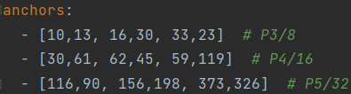
下面是yolov5 v7.0中的anchor,这是在coco数据集上通过聚类方法得到的。当我们的输入尺寸为640*640时,会得到3个不同尺度的输出:80x80(640/8)、40x40(640/16)、20x20(640/32)。其中,80x80代表浅层的特征图(P3),包含较多的低层级信息,适合用于检测小目标,所以这一特征图所用的anchor尺度较小;20x20代表深层的特征图(P5),包含更多高层级的信息,如轮廓、结构等信息,适合用于大目标的检测,所以这一特征图所用的anchor尺度较大。另外的40x40特征图(P4)上就用介于这两个尺度之间的anchor用来检测中等大小的目标。对于20*20尺度大小的特征图,由原图下采样32倍得到,因此先验框由640*640尺度下的 (116 × 90), (156 × 198),(373 × 326) 缩小32倍,变成 (3.625× 2.8125), (4.875× 6.1875),(11.6563×10.1875),其共有13*13个grid cell,则这每个169个grid cell都会被分配3*13*13个先验框。
在Yolov3、Yolov4中,训练不同的数据集时,计算初始锚框的值是通过单独的程序运行的。但Yolov5中将此功能嵌入到代码中,每次训练时,自适应的计算不同训练集中的最佳锚框值。当然,如果觉得计算的锚框效果不是很好,也可以在train.py中将自动计算锚框功能关闭。
![]()
Yolov5的自适应锚框计算函数kmean_anchors(位于utils/autoanchor.py)
def kmean_anchors(path='./data/coco128.yaml', n=9, img_size=640, thr=4.0, gen=1000, verbose=True):
    """在check_anchors中调用
    使用K-means + 遗传算法 算出更符合当前数据集的anchors
    Creates kmeans-evolved anchors from training dataset
    :params path: 数据集的路径/数据集本身
    :params n: anchors 的个数
    :params img_size: 数据集图片约定的大小
    :params thr: 阈值 由 hyp['anchor_t'] 参数控制
    :params gen: 遗传算法进化迭代的次数(突变 + 选择)
    :params verbose: 是否打印所有的进化(成功的)结果 默认传入是False, 只打印最佳的进化结果
    :return k: K-means + 遗传算法进化后的anchors
    """
    from scipy.cluster.vq import kmeans


    # 注意一下下面的thr不是传入的thr,而是1/thr, 所以在计算指标这方面还是和check_anchor一样
    thr = 1. / thr  # 0.25
    prefix = colorstr('autoanchor: ')

    def metric(k, wh):  # compute metrics
        """用于 print_results 函数和 anchor_fitness 函数
        计算ratio metric: 整个数据集的  ground truth 框与 anchor 对应宽比和高比即:gt_w/k_w,gt_h/k_h + x + best_x  用于后续计算BPR+aat
        注意我们这里选择的metric是 ground truth 框与anchor对应宽比和高比 而不是常用的iou 这点也与nms的筛选条件对应 是yolov5中使用的新方法
        :params k: anchor框
        :params wh: 整个数据集的 wh [N, 2]
        :return x: [N, 9] N 个 ground truth 框与所有 anchor 框的宽比或高比(两者之中较小者)
        :return x.max(1)[0]: [N] N个 ground truth 框与所有 anchor 框中的最大宽比或高比(两者之中较小者)
        """
        # [N, 1, 2] / [1, 9, 2] = [N, 9, 2]  N个gt_wh和9个anchor的k_wh宽比和高比
        # 两者的重合程度越高 就越趋近于1 远离1(<1 或 >1)重合程度都越低
        r = wh[:, None] / k[None]
        # r=gt_height/anchor_height  gt_width / anchor_width  有可能大于1,也可能小于等于1
        # flow.min(r, 1. / r): [N, 9, 2] 将所有的宽比和高比统一到 <=1
        # .min(2): value=[N, 9] 选出每个 ground truth 个和 anchor 的宽比和高比最小的值   index: [N, 9] 这个最小值是宽比(0)还是高比(1)
        # [0] 返回 value [N, 9]  每个 ground truth 个和 anchor 的宽比和高比最小的值 就是所有 ground truth 与 anchor 重合程度最低的
        x = flow.min(r, 1. / r).min(2)[0]  # ratio metric
        # x = wh_iou(wh, flow.tensor(k))  # IoU metric
        # x.max(1)[0]: [N] 返回每个 ground truth 和所有 anchor(9个) 中宽比/高比最大的值
        return x, x.max(1)[0]  # x, best_x

    def anchor_fitness(k):   # mutation fitness
        """用于 kmean_anchors 函数
        适应度计算 优胜劣汰 用于遗传算法中衡量突变是否有效的标注 如果有效就进行选择操作,无效就继续下一轮的突变
        :params k: [9, 2] K-means生成的 9 个anchors     wh: [N, 2]: 数据集的所有 ground truth 框的宽高
        :return (best * (best > thr).float()).mean()=适应度计算公式 [1] 注意和BPR有区别 这里是自定义的一种适应度公式
                返回的是输入此时anchor k 对应的适应度
        """
        _, best = metric(flow.tensor(k, dtype=flow.float32), wh)
        return (best * (best > thr).float()).mean()  # fitness

    def print_results(k):
        """用于 kmean_anchors 函数中打印K-means计算相关信息
        计算BPR、aat=>打印信息: 阈值+BPR+aat  anchor个数+图片大小+metric_all+best_mean+past_mean+Kmeans聚类出来的anchor框(四舍五入)
        :params k: K-means得到的anchor k
        :return k: input
        """
        # 将K-means得到的anchor k按面积从小到大排序
        k = k[np.argsort(k.prod(1))]
        # x: [N, 9] N个 ground truth 框与所有anchor框的宽比或高比(两者之中较小者)
        # best: [N] N个 ground truth 框与所有anchor框中的最大宽比或高比(两者之中较小者)
        x, best = metric(k, wh0)
        # (best > thr).float(): True=>1.  False->0.  .mean(): 求均值
        # BPR(best possible recall): 最多能被召回(通过thr)的 ground truth 框数量 / 所有 ground truth 框数量  [1] 0.96223  小于0.98 才会用K-means计算anchor
        # aat(anchors above threshold): [1] 3.54360 每个target平均有多少个anchors
        BPR, aat = (best > thr).float().mean(), (x > thr).float().mean() * n  # best possible recall, anch > thr
        f = anchor_fitness(k)
        # print(f'{prefix}thr={thr:.2f}: {BPR:.4f} best possible recall, {aat:.2f} anchors past thr')
        # print(f'{prefix}n={n}, img_size={img_size}, metric_all={x.mean():.3f}/{best.mean():.3f}-mean/best, '
        #       f'past_thr={x[x > thr].mean():.3f}-mean: ', end='')
        print(f"aat: {aat:.5f}, fitness: {f:.5f}, best possible recall: {BPR:.5f}")
        for i, x in enumerate(k):
            print('%i,%i' % (round(x[0]), round(x[1])), end=',  ' if i < len(k) - 1 else '\n')  # use in *.cfg

        return k


    # 载入数据集
    if isinstance(path, str):  # *.yaml file
        with open(path) as f:
            data_dict = yaml.safe_load(f)  # model dict
        from utils.datasets import LoadImagesAndLabels
        dataset = LoadImagesAndLabels(data_dict['train'], augment=True, rect=True)
    else:
        dataset = path  # dataset

    # 得到数据集中所有数据的 wh
    # 将数据集图片的最长边缩放到 img_size, 较小边相应缩放
    shapes = img_size * dataset.shapes / dataset.shapes.max(1, keepdims=True)
    # 将原本数据集中gt boxes归一化的wh缩放到shapes尺度
    wh0 = np.concatenate([l[:, 3:5] * s for s, l in zip(shapes, dataset.labels)])

    # 统计gt boxes中宽或者高小于 3 个像素的个数, 目标太小 发出警告
    i = (wh0 < 3.0).any(1).sum()
    if i:
        print(f'{prefix}WARNING: Extremely small objects found. {i} of {len(wh0)} labels are < 3 pixels in size.')

    # 筛选出 label 大于 2 个像素的框拿来聚类, [...]内的相当于一个筛选器, 为True的留下
    wh = wh0[(wh0 >= 2.0).any(1)]  # filter > 2 pixels
    # wh = wh * (np.random.rand(wh.shape[0], 1) * 0.9 + 0.1)  # multiply by random scale 0-1

    # Kmeans聚类方法: 使用欧式距离来进行聚类
    print(f'{prefix}Running kmeans for {n} anchors on {len(wh)} gt boxes...')
    # 计算宽和高的标准差->[w_std,h_std]
    s = wh.std(0)  # sigmas for whitening
    # 开始聚类,仍然是聚成 n 类,返回聚类后的anchors k(这个anchors k是白化后数据的anchor框s)
    # 另外还要注意的是这里的kmeans使用欧式距离来计算的
    # 运行K-means的次数为30次  obs: 传入的数据必须先白化处理 'whiten operation'
    # 白化处理: 新数据的标准差=1 降低数据之间的相关度,不同数据所蕴含的信息之间的重复性就会降低,网络的训练效率就会提高
    # 白化操作参考博客: https://blog.csdn.net/weixin_37872766/article/details/102957235
    k, dist = kmeans(wh / s, n, iter=30)  # points, mean distance
    assert len(k) == n, print(f'{prefix}ERROR: scipy.cluster.vq.kmeans requested {n} points but returned only {len(k)}')
    k *= s  # k*s 得到原来数据(白化前)的 anchor 框

    wh = flow.tensor(wh, dtype=flow.float32)  # filtered wh
    wh0 = flow.tensor(wh0, dtype=flow.float32)  # unfiltered wh0

    # 输出新算的anchors k 相关的信息
    k = print_results(k)

    # Plot wh
    # k, d = [None] * 20, [None] * 20
    # for i in tqdm(range(1, 21)):
    #     k[i-1], d[i-1] = kmeans(wh / s, i)  # points, mean distance
    # fig, ax = plt.subplots(1, 2, figsize=(14, 7), tight_layout=True)
    # ax = ax.ravel()
    # ax[0].plot(np.arange(1, 21), np.array(d) ** 2, marker='.')
    # fig, ax = plt.subplots(1, 2, figsize=(14, 7))  # plot wh
    # ax[0].hist(wh[wh[:, 0]<100, 0], 400)
    # ax[1].hist(wh[wh[:, 1]<100, 1], 400)
    # fig.savefig('wh.png', dpi=200)

    # Evolve 类似遗传/进化算法  变异操作
    npr = np.random   # 随机工具
    # f: fitness 0.62690
    # sh: (9,2)
    # mp: 突变比例mutation prob=0.9   s: sigma=0.1
    f, sh, mp, s = anchor_fitness(k), k.shape, 0.9, 0.1  # fitness, generations, mutation prob, sigma
    pbar = tqdm(range(gen), desc=f'{prefix}Evolving anchors with Genetic Algorithm:')  # progress bar
    # 根据聚类出来的n个点采用遗传算法生成新的anchor
    for _ in pbar:
        # 重复1000次突变+选择 选择出1000次突变里的最佳anchor k和最佳适应度f
        v = np.ones(sh)  # v [9, 2] 全是1
        while (v == 1).all():
            # 产生变异规则 mutate until a change occurs (prevent duplicates)
            # npr.random(sh) < mp: 让v以90%的比例进行变异  选到变异的就为1  没有选到变异的就为0
            v = ((npr.random(sh) < mp) * npr.random() * npr.randn(*sh) * s + 1).clip(0.3, 3.0)
        # 变异(改变这一时刻之前的最佳适应度对应的anchor k)
        kg = (k.copy() * v).clip(min=2.0)
        # 计算变异后的anchor kg的适应度
        fg = anchor_fitness(kg)
        # 如果变异后的anchor kg的适应度>最佳适应度k 就进行选择操作
        if fg > f:
            # 选择变异后的anchor kg为最佳的anchor k 变异后的适应度fg为最佳适应度f
            f, k = fg, kg.copy()

            # 打印信息
            pbar.desc = f'{prefix}Evolving anchors with Genetic Algorithm: fitness = {f:.4f}'
            if verbose:
                print_results(k)
    return print_results(k)
1.3 自适应图片缩放
在常用的目标检测算法中,不同的图片长宽都不相同,因此常用的方式是将原始图片缩放填充到标准尺寸,再送入检测网络中。在项目实际使用时,很多图片的长宽比不同,因此缩放填充后,两端的黑边大小都不同,而如果填充的比较多,则存在信息冗余,影响推理速度。因此在Yolov5的代码中utils/augmentations.py的letterbox函数中进行了修改,对原始图像自适应的添加最少的黑边。
Yolov5的letterbox函数(utils/augmentations.py)
假设图片原来尺寸为(1080, 1920),我们想要resize的尺寸为(640,640)。要想满足收缩的要求,640/1080= 0.59,640/1920 = 0.33,应该选择更小的收缩比例0.33,则图片被缩放为(360,640)。下一步则要填充灰白边至360可以被32整除,则应该填充至384,最终得到图片尺寸(384,640)。
def letterbox(im, new_shape=(640, 640), color=(114, 114, 114), auto=True, scaleFill=False, scaleup=True, stride=32):
    # Resize and pad image while meeting stride-multiple constraints
    shape = im.shape[:2]  # current shape [height, width] 当前图像尺寸
    if isinstance(new_shape, int):
        new_shape = (new_shape, new_shape)  # 缩放后的尺寸

    # Scale ratio (new / old) 计算缩放比例(选择长宽中更小的那个缩放比例)
    r = min(new_shape[0] / shape[0], new_shape[1] / shape[1])
    if not scaleup:  # only scale down, do not scale up (for better val mAP)
        r = min(r, 1.0)

    # Compute padding
    ratio = r, r  # width, height ratios
    new_unpad = int(round(shape[1] * r)), int(round(shape[0] * r))  # 直接缩放后的宽高
    dw, dh = new_shape[1] - new_unpad[0], new_shape[0] - new_unpad[1]  # wh padding 计算灰边填充数值
    if auto:  # minimum rectangle 采用自适应图片缩放,确保宽和高都能被stride整除,因此需要补边
        dw, dh = np.mod(dw, stride), np.mod(dh, stride)  # wh padding 取余np.mod
    elif scaleFill:  # stretch  不采用自适应缩放,直接resize到目标shape,无需补边
        dw, dh = 0.0, 0.0
        new_unpad = (new_shape[1], new_shape[0])
        ratio = new_shape[1] / shape[1], new_shape[0] / shape[0]  # width, height ratios

    dw /= 2  # divide padding into 2 sides
    dh /= 2  # 上下和左右两侧各 padding 一半

    if shape[::-1] != new_unpad:  # resize
        im = cv2.resize(im, new_unpad, interpolation=cv2.INTER_LINEAR)
    top, bottom = int(round(dh - 0.1)), int(round(dh + 0.1))  # 上下两侧需要padding的大小
    left, right = int(round(dw - 0.1)), int(round(dw + 0.1))  # 左右两侧需要padding的大小
    im = cv2.copyMakeBorder(im, top, bottom, left, right, cv2.BORDER_CONSTANT, value=color)  # add border 填充114
    return im, ratio, (dw, dh)
2 BackBone
- YOLOv1的Backbone总共24个卷积层和2个全连接层,使用了Leaky ReLu激活函数,但并没有引入BN层。
- YOLOv2的Backbone在YOLOv1的基础上设计了Darknet-19网络,包含19个卷积层并引入了BN层优化模型整体性能。
- YOLOv3将YOLOv2的Darknet-19加深了网络层数,并引入了ResNet的残差思想,也正是残差思想让YOLOv3将Backbone深度大幅扩展至Darknet-53。
- YOLOv4的Backbone在YOLOv3的基础上,受CSPNet网络结构启发,将多个CSP子模块进行组合设计成为CSPDarknet53,并且使用了Mish激活函数(除Backbone以外的网络结构依旧使用LeakyReLU激活函数)。CSPDarknet53总共有72层卷积层,遵循YOLO系列一贯的风格,这些卷积层都是3*3 大小,步长为2的设置,能起到特征提取与逐步下采样的作用。
- YOLOv5的Backbone同样使用了YOLOv4中使用的CSP思想。YOLOv5最初版本中会存在Focus结构,在YOLOv5第六版开始后,就舍弃了这个结构改用常规卷积,其产生的参数更少,效果更好。
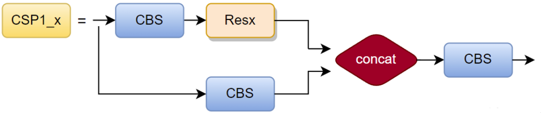
2.1 CSP
CSP结构的核心思想是将输入特征图分成两部分,一部分经过一个小的卷积网络(称为子网络)进行处理,另一部分则直接进行下一层的处理。然后将两部分特征图拼接起来,作为下一层的输入。Yolov4和Yolov5都使用了CSP结构,yolov4只在backbone中使用了CSP结构,yolov5有两种CSP结构,以Yolov5s网络为例,CSP1_X结构应用于Backbone主干网络,另一种CSP2_X结构则应用于Neck中。残差组件由两个CBL组成,因此两个CSP的区别在于有没有shortcut(通过BottleneckCSP类的shortcut参数设置)。
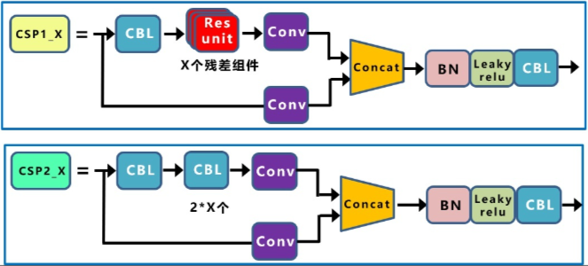
在YOLOv5 v4.0中,作者将BottleneckCSP模块转变为了C3模块,经历过残差输出后的Conv模块被去掉了。C3包含了3个标准卷积层以及多个Bottleneck模块(数量由配置文件.yaml的n和depth_multiple参数乘积决定),concat后的标准卷积模块中的激活函数也由LeakyRelu变为了SiLU。
YOLOv5中的C3类
class Bottleneck(nn.Module):
    # Standard bottleneck
    def __init__(self, c1, c2, shortcut=True, g=1, e=0.5):  # ch_in, ch_out, shortcut, groups, expansion
        super().__init__()
        c_ = int(c2 * e)  # hidden channels
        self.cv1 = Conv(c1, c_, 1, 1)
        self.cv2 = Conv(c_, c2, 3, 1, g=g)
        self.add = shortcut and c1 == c2

    def forward(self, x):
        return x + self.cv2(self.cv1(x)) if self.add else self.cv2(self.cv1(x))

class C3(nn.Module):
    # CSP Bottleneck with 3 convolutions
    def __init__(self, c1, c2, n=1, shortcut=True, g=1, e=0.5):  # ch_in, ch_out, number, shortcut, groups, expansion
        super().__init__()
        c_ = int(c2 * e)  # hidden channels
        self.cv1 = Conv(c1, c_, 1, 1)   # Conv = conv+BN+SiLU
        self.cv2 = Conv(c1, c_, 1, 1)
        self.cv3 = Conv(2 * c_, c2, 1)  # optional act=FReLU(c2)
        self.m = nn.Sequential(*(Bottleneck(c_, c_, shortcut, g, e=1.0) for _ in range(n)))  # 串联n个残差结构
        # self.m = nn.Sequential(*(CrossConv(c_, c_, 3, 1, g, 1.0, shortcut) for _ in range(n)))

    def forward(self, x):
        return self.cv3(torch.cat((self.m(self.cv1(x)), self.cv2(x)), 1))
3 Neck
- yolov1、yolov2没有使用Neck模块,yolov3开始使用。Neck模块的目的是融合不同层的特征检测大中小目标。
- yolov3的NECK模块引入了FPN的思想,并对原始FPN进行修改。
- yolov4的Neck模块主要包含了SPP模块和PAN模块。SPP,即空间金字塔池化。SPP的目的是解决了输入数据大小任意的问题。SPP网络用在YOLOv4中的目的是增加网络的感受野。
- yolov5的Neck侧也使用了SPP模块和PAN模块,但是在PAN模块进行融合后,将YOLOv4中使用的CBL模块替换成借鉴CSPnet设计的CSP_v5结构,加强网络特征融合的能力。
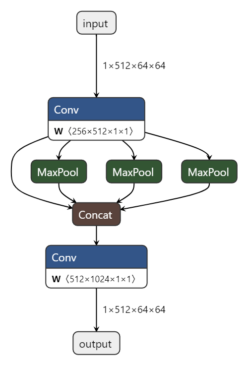
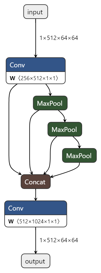
3.1 SPP/SPPF
2014年何恺明提出了空间金字塔池化SPP,能将任意大小的特征图转换成固定大小的特征向量。在Yolov5中,SPP的目的是在不同尺度下对图像进行池化(Pooling)。这种结构可以在不同尺寸的特征图上利用ROI池化不同尺度下的特征信息,提高模型的精度和效率。在YOLOv5的实现中,SPP结构主要包含两个版本,分别为SPP和SPPF。其中,SPP代表“Spatial Pyramid Pooling”,而SPPF则代表“Fast Spatial Pyramid Pooling”。两者目的是相同的,只是在结构上略有差异,从SPP改进为SPPF后(Yolov5 6.0),模型的计算量变小了很多,模型速度提升。结构图如下图所示,下面的Conv是CBS=conv+BN+SiLU。
YOLOv5中的SPP/SPPF类
class SPP(nn.Module):
    # Spatial Pyramid Pooling (SPP) layer https://arxiv.org/abs/1406.4729
    def __init__(self, c1, c2, k=(5, 9, 13)):  # 5, 9, 13为初始化的kernel size
        super().__init__()
        c_ = c1 // 2  # hidden channels
        self.cv1 = Conv(c1, c_, 1, 1)          # 通道减半
        self.cv2 = Conv(c_ * (len(k) + 1), c2, 1, 1)  # concat之后的CBS
        self.m = nn.ModuleList([nn.MaxPool2d(kernel_size=x, stride=1, padding=x // 2) for x in k])

    def forward(self, x):
        x = self.cv1(x)
        with warnings.catch_warnings():
            warnings.simplefilter('ignore')  # suppress torch 1.9.0 max_pool2d() warning
            return self.cv2(torch.cat([x] + [m(x) for m in self.m], 1))


class SPPF(nn.Module):
    # Spatial Pyramid Pooling - Fast (SPPF) layer for YOLOv5 by Glenn Jocher
    def __init__(self, c1, c2, k=5):  # equivalent to SPP(k=(5, 9, 13))
        super().__init__()
        c_ = c1 // 2  # hidden channels
        self.cv1 = Conv(c1, c_, 1, 1)
        self.cv2 = Conv(c_ * 4, c2, 1, 1)
        self.m = nn.MaxPool2d(kernel_size=k, stride=1, padding=k // 2)

    def forward(self, x):
        x = self.cv1(x)
        with warnings.catch_warnings():
            warnings.simplefilter('ignore')  # suppress torch 1.9.0 max_pool2d() warning
            y1 = self.m(x)
            y2 = self.m(y1) # 串联k=5的池化,会获得9和13的池化,所以是等效的,但是时间更快
            return self.cv2(torch.cat((x, y1, y2, self.m(y2)), 1))
3.2 PAN
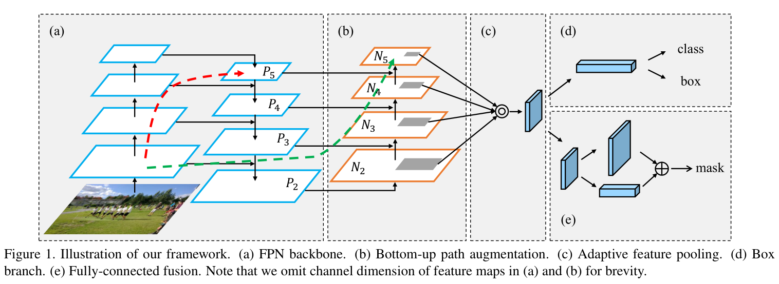
论文:Path Aggregation Network for Instance Segmentation
PANet是香港中文大学 2018 作品,在COCO2017的实例分割上获得第一,在目标检测任务上获得第二。作者通过研究Mask R-CNN发现底层特征难以传达到高层次,因此设计了自下而上的路径增强,如下图里的(b)所示,(c)是Adaptive feature pooling。红色线表达了图像底层特征在FPN中的传递路径,要经过100多层layers;绿色线表达了图像底层特征在PANnet 中的传递路径,只需要经过小于10层layers。
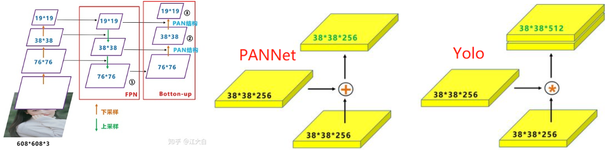
Yolov5中的PAN结构
FPN层自顶向下传达强语义特征(高层语义是经过特征提取后得到的特征信息,它的感受野较大,提取的特征抽象,有利于物体的分类,但会丢失细节信息,不利于精确分割。高层语义特征是抽象的特征)。而PAN则自底向上传达强定位特征,两两联手,从不同的主干层对不同的检测层进行参数聚合。原本的PANet网络的PAN结构中,两个特征图结合是采用shortcut操作,而Yolov4/5中则采用concat操作,特征图融合后的尺寸发生了变化。
4 输出端
4.1 正样本采样
什么是正负样本?
正负样本都是针对于算法经过处理生成的框,用于计算损失,而在预测过程和验证过程是没有这个概念的。正例用来使预测结果更靠近真实值的,负例用来使预测结果更远离除了真实值之外的值的。正负样本的比例最好为1:1到1:2左右,数量差距不能太悬殊,特别是正样本数量本来就不太多的情况下。如果负样本远多于正样本,则负样本会淹没正样本的损失,从而降低网络收敛的效率与检测精度。这就是目标检测中常见的正负样本不均衡问题,解决方案之一是增加正样本数。
yolov5通过以下三个方法增加正样本数量:
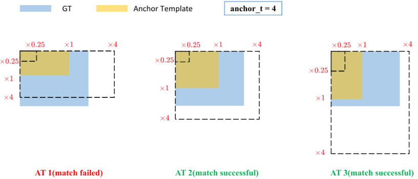
(1) 跨anchor预测
假设一个GT框落在了某个预测分支的某个网格内,该网格具有3种不同大小anchor,若GT可以和这3种anchor中的多种anchor匹配,则这些匹配的anchor都可以来预测该GT框,即一个GT框可以使用多种anchor来预测。预测边框的宽高是基于anchor来预测的,而预测的比例值是有范围的,即0-4,如果标签的真实宽高与anchor的宽高的比例超过了4,那是不可能预测成功的,所以哪些anchor能匹配上哪些标签,就看anchor的宽(高)与标签的宽(高)的比例有没有超过4,如果超过了,那就不匹配。注意,这个比例是双向的比例,比如标签宽/anchor宽>4,不匹配,而anchor宽/标签宽>4,也是不匹配的。
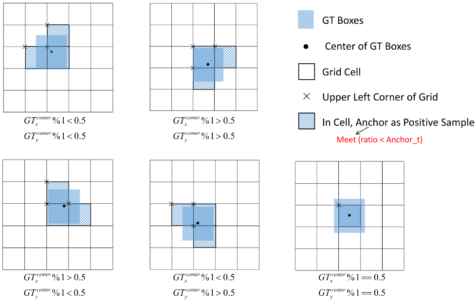
(2) 跨grid预测
假设一个GT框落在了某个预测分支的某个网格内,则该网格有左、上、右、下4个邻域网格,根据GT框的中心位置,将最近的2个邻域网格也作为预测网格,也即一个GT框可以由3个网格来预测。有下面5种情况(如果标签边框的中心点正好落在格子中间,就只有这个格子了):
(3) 跨分支预测
假设一个GT框可以和2个甚至3个预测分支上的anchor匹配,则这2个或3个预测分支都可以预测该GT框,即一个GT框可以由多个预测分支来预测,重复anchor匹配和grid匹配的步骤,可以得到某个GT 匹配到的所有正样本。
yolov5的正样本匹配:即找到与targets对应的所有正样本
    def build_targets(self, p, targets):
        # Build targets for compute_loss(), input targets(image,class,x,y,w,h)
        na, nt = self.na, targets.shape[0]  # na为类别数,nt为目标数
        tcls, tbox, indices, anch = [], [], [], []
        gain = torch.ones(7, device=self.device)  # normalized to gridspace gain
        ai = torch.arange(na, device=self.device).float().view(na, 1).repeat(1, nt)  # ai.shape = (na, nt),锚框的索引,第二个维度复制nt遍
        targets = torch.cat((targets.repeat(na, 1, 1), ai[..., None]), 2)  # targets.shape = (na, nt, 7)给每个目标加上锚框索引

        g = 0.5  # bias
        off = torch.tensor(
            [
                [0, 0],
                [1, 0],
                [0, 1],
                [-1, 0],
                [0, -1],  # j,k,l,m
                # [1, 1], [1, -1], [-1, 1], [-1, -1],  # jk,jm,lk,lm
            ],
            device=self.device).float() * g  # offsets

        for i in range(self.nl):  # self.nl为预测层也就是检测头的数量,anchor匹配需要逐层进行
            anchors = self.anchors[i]  # 该预测层上的anchor尺寸,三个尺寸
            gain[2:6] = torch.tensor(p[i].shape)[[3, 2, 3, 2]]  # 比如在P3层 gain=tensor([ 1.,  1., 80., 80., 80., 80.,  1.], device='cuda:0')

            # Match targets to anchors
            t = targets * gain  # shape(3,n,7) 将归一化的gtbox乘以特征图尺度,将box坐标投影到特征图上
            if nt:
                # Matches
                r = t[..., 4:6] / anchors[:, None]  # 计算标签box和当前层的anchors的宽高比,即:wb/wa,hb/ha
                j = torch.max(r, 1 / r).max(2)[0] < self.hyp['anchor_t']  # 将比值和预先设置的比例anchor_t对比,符合条件为True,反之False
                # j = wh_iou(anchors, t[:, 4:6]) > model.hyp['iou_t']  # iou(3,n)=wh_iou(anchors(3,2), gwh(n,2))
                t = t[j]  # 筛选出符合条件target

                # Offsets
                gxy = t[:, 2:4]  # 得到相对于以左上角为坐标原点的坐标                          假设某个gt的中心点为gxy=[22.20, 19.05]
                gxi = gain[[2, 3]] - gxy  # 得到相对于右下角为坐标原点的坐标                   此时gxi=[17.80, 20.95]
                j, k = ((gxy % 1 < g) & (gxy > 1)).T  # jk判断gxy的中心点是否更偏向左上角     g=0.5 操作%1得到小数部分,小于0.5,所以j,k均为True
                l, m = ((gxi % 1 < g) & (gxi > 1)).T  # lm判断gxy的中心点是否更偏向右下角     g=0.5 l,m均为False,该舞台中心更偏向于左上角
                j = torch.stack((torch.ones_like(j), j, k, l, m))  # 网格本身是True,再加上 上下左右
                t = t.repeat((5, 1, 1))[j]  # 这里将t复制5个,然后使用j来过滤
                offsets = (torch.zeros_like(gxy)[None] + off[:, None])[j]
            else:
                t = targets[0]
                offsets = 0

            # Define
            bc, gxy, gwh, a = t.chunk(4, 1)  # (image, class), grid xy, grid wh, anchors
            a, (b, c) = a.long().view(-1), bc.long().T  # anchors, image, class 其中,a表示当前gt box和当前层的第几个anchor匹配上了
            gij = (gxy - offsets).long()  # .long()为取整 gij是gxy的整数部分
            gi, gj = gij.T  # grid indices (gi,gj)是我们计算出来的负责预测该gt box的网格的坐标。

            # Append
            # indices中是正样本所对应的gt的信息  b表示当前正样本对应的gt属于该batch内第几张图片,a表示gtbox与anchors的对应关系,gj负责预测的网格纵坐标,gi负责预测的网格横坐标
            indices.append((b, a, gj.clamp_(0, gain[3] - 1), gi.clamp_(0, gain[2] - 1)))  # image, anchor, grid indices
            # tbox, anch, tcls是正样本自己的信息
            tbox.append(torch.cat((gxy - gij, gwh), 1))  # 正样本相对网格的偏移,宽高
            anch.append(anchors[a])  # 正样本对应的anchor信息
            tcls.append(c)  # 正样本的类别信息

        return tcls, tbox, indices, anch
4.2 损失计算
Yolov5官方文档:https://docs.ultralytics.com/yolov5/tutorials/architecture_description/?h=loss#3-training-strategies
损失函数的调用点如下,在train.py中
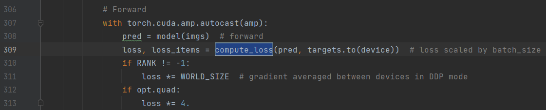
pre:网络从三个特征图上得到3*(20*20+40*40+52*52)个先验框,每个先验框由6个参数:px,py,pw,ph,po和pcls
targets:一个batch中所有的目标(如果开启开启mosaic数据增强的话,每张图就包含原本多张图中的目标),每个目标有(image,class,x,y,w,h)共6个参数,shape=[ num,6]。
损失函数分三部分:(1)分类损失Lcls (BCE loss) (2)置信度损失Lobj(BCE loss) (3)边框损失Lloc(CIOU loss)
![]()
其中置信度损失在三个预测层(P3, P4, P5)上权重不同,分别为[4.0, 1.0, 0.4]
![]()
这三者的权重都是可以设置的,在默认的data/hyps/hyp.scratch-low.yaml中,如下图
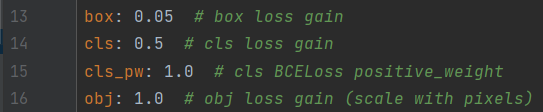
这三个损失权重会根据类别、图像大小、检测层数量进行scale

4.2.1 分类损失
按照640乘640分辨率,3个输出层来算的话,P3是80乘80个格子,P4是40乘40,P5是20乘20,一共有8400个格子,并不是每一个格子上的输出都要去做分类损失计算的,只有负责预测对应物体的格子才需要做分类损失计算(边框损失计算也是一样)。
分类损失采用nn.BCEWithLogitsLoss,即二分类损失,比如现在有4个分类:猫、狗、猪、鸡,当前标签真值为猪,那么计算损失的时候,targets就是[0, 0, 1, 0],推理结果的分类部分也会有4个值,分别是4个分类的概率,就相当于计算4次二分类损失,取均值。分类的真值也不一定是0或1,因为可以做label smoothing。
# Classification
if self.nc > 1:  # cls loss (only if multiple classes)
    t = torch.full_like(pcls, self.cn, device=self.device)  # torch.full_like返回一个形状与pcls相同且值全为self.cn的张量
    t[range(n), tcls[i]] = self.cp  # 对应类别处为self.cp, 其余类别处为self.cn
    lcls += self.BCEcls(pcls, t)  # BCE
4.2.2 置信度损失
每一个格子都要计算置信度损失,置信度的真值并不是固定的,如果该格子负责预测对应的物体,那么置信度真值就是预测边框与标签边框的IOU。如果不负责预测任何物体,那真值就是0。
与早期版本的YOLO相比,YOLOv5架构对预测框策略进行了更改。在YOLOv2和YOLOv3中,使用最后一层的激活直接预测框坐标。如下图所示
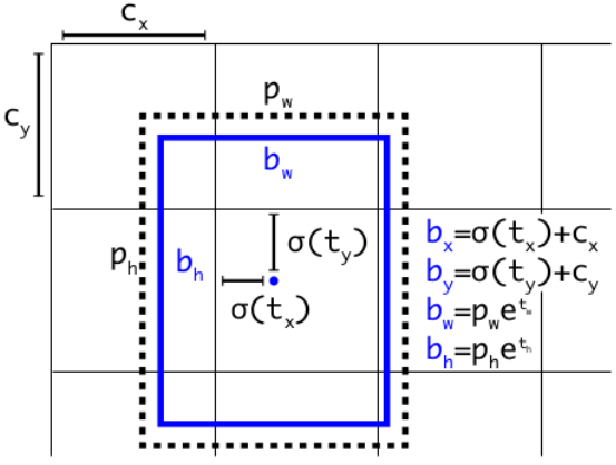
而在YOLOv5中,用于预测框坐标的公式已经更新,以降低网格灵敏度,并防止模型预测没有边界。计算预测边界框的修订公式如下:
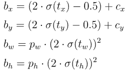
Yolov5预测框坐标计算,以与target的iou计算
                # pxy, pwh, _, pcls = pi[b, a, gj, gi].tensor_split((2, 4, 5), dim=1)  # faster, requires torch 1.8.0
                pxy, pwh, _, pcls = pi[b, a, gj, gi].split((2, 2, 1, self.nc), 1)  # target-subset of predictions

                # Regression
                pxy = pxy.sigmoid() * 2 - 0.5
                pwh = (pwh.sigmoid() * 2) ** 2 * anchors[i]
                pbox = torch.cat((pxy, pwh), 1)  # predicted box
                iou = bbox_iou(pbox, tbox[i], CIoU=True).squeeze()  # iou(prediction, target)
                lbox += (1.0 - iou).mean()  # iou loss

                # Objectness
                iou = iou.detach().clamp(0).type(tobj.dtype)
                if self.sort_obj_iou:
                    j = iou.argsort()
                    b, a, gj, gi, iou = b[j], a[j], gj[j], gi[j], iou[j]
                if self.gr < 1:
                    iou = (1.0 - self.gr) + self.gr * iou
                tobj[b, a, gj, gi] = iou  # iou ratio
4.2.3 边框损失
Bounding Box Regeression的Loss近些年的发展过程是:Smooth L1 Loss-> IoU Loss(2016)-> GIoU Loss(2019)-> DIoU Loss(2020)->CIoU Loss(2020),Yolov5用的是CIOU。
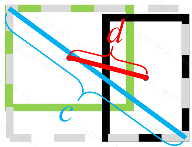
![]()
其中,ρ预测框和真实框的中心点的欧式距离,也就是图中的d,c代表的是能够同时包含预测框和真实框的最小闭包区域的对角线距离,v测量纵横比的一致性,α是正的权衡参数,
![]()
![]()
Yolov5中IOU、CIoU、DIoU、GIoU的计算
论文:Distance-IoU Loss: Faster and Better Learning for Bounding Box Regression
def bbox_iou(box1, box2, xywh=True, GIoU=False, DIoU=False, CIoU=False, eps=1e-7):
    # Returns Intersection over Union (IoU) of box1(1,4) to box2(n,4)

    # Get the coordinates of bounding boxes
    if xywh:  # transform from xywh to xyxy
        (x1, y1, w1, h1), (x2, y2, w2, h2) = box1.chunk(4, 1), box2.chunk(4, 1)
        w1_, h1_, w2_, h2_ = w1 / 2, h1 / 2, w2 / 2, h2 / 2
        b1_x1, b1_x2, b1_y1, b1_y2 = x1 - w1_, x1 + w1_, y1 - h1_, y1 + h1_
        b2_x1, b2_x2, b2_y1, b2_y2 = x2 - w2_, x2 + w2_, y2 - h2_, y2 + h2_
    else:  # x1, y1, x2, y2 = box1
        b1_x1, b1_y1, b1_x2, b1_y2 = box1.chunk(4, 1)
        b2_x1, b2_y1, b2_x2, b2_y2 = box2.chunk(4, 1)
        w1, h1 = b1_x2 - b1_x1, b1_y2 - b1_y1 + eps
        w2, h2 = b2_x2 - b2_x1, b2_y2 - b2_y1 + eps

    # Intersection area
    inter = (torch.min(b1_x2, b2_x2) - torch.max(b1_x1, b2_x1)).clamp(0) * \
            (torch.min(b1_y2, b2_y2) - torch.max(b1_y1, b2_y1)).clamp(0)

    # Union Area
    union = w1 * h1 + w2 * h2 - inter + eps

    # IoU
    iou = inter / union
    if CIoU or DIoU or GIoU:
        cw = torch.max(b1_x2, b2_x2) - torch.min(b1_x1, b2_x1)  # convex (smallest enclosing box) width
        ch = torch.max(b1_y2, b2_y2) - torch.min(b1_y1, b2_y1)  # convex height
        if CIoU or DIoU:  # Distance or Complete IoU https://arxiv.org/abs/1911.08287v1
            c2 = cw ** 2 + ch ** 2 + eps  # convex diagonal squared
            rho2 = ((b2_x1 + b2_x2 - b1_x1 - b1_x2) ** 2 + (b2_y1 + b2_y2 - b1_y1 - b1_y2) ** 2) / 4  # center dist ** 2
            if CIoU:  # https://github.com/Zzh-tju/DIoU-SSD-pytorch/blob/master/utils/box/box_utils.py#L47
                v = (4 / math.pi ** 2) * torch.pow(torch.atan(w2 / h2) - torch.atan(w1 / h1), 2)
                with torch.no_grad():
                    alpha = v / (v - iou + (1 + eps))
                return iou - (rho2 / c2 + v * alpha)  # CIoU
            return iou - rho2 / c2  # DIoU
        c_area = cw * ch + eps  # convex area
        return iou - (c_area - union) / c_area  # GIoU https://arxiv.org/pdf/1902.09630.pdf
    return iou  # IoU
参考:
5. 复制-粘贴大法(Copy-Paste):简单而有效的数据增强
6. 数据增强mixup技术