(一).选题背景:
什么是图像分类?它有哪些应用场合?图像分类任务是计算机视觉中的核心任务,其目标是根据图像信息中所反映的不同特征,把不同类别的图像区分开来。从已知的类别标签集合中为给定的输入图片选定一个类别标签。
它的难点在于:跨越“语义鸿沟”建立像素到语义的映射。还有就是视角、光照、尺度、遮挡、形变、背景杂波、类内形变、运动模糊、类别繁多等问题。
手机拍照、智能安防、自动驾驶等场景有广泛应用。从2012年AlexNet在ImageNet比赛夺冠以来,深度学习深刻推动了计算机视觉领域的发展,当前最先进的计算机视觉算法几乎都是深度学习相关的。深度神经网络可以逐层提取图像特征,并保持局部不变性,被广泛应用于分类、检测、分割、检索、识别、提升、重建等视觉任务中。
数据来源:kaggle,网址:https//www.kaggle.com/
(二).机器学习的实验步骤:
1. 关于数据
20类头饰的图像级—帽子、便帽。
3620幅训练图像、100幅验证图像
所以图像都是224*224*3的jpg格式
2. 导入库
try:
  # %tensorflow_version 仅存在于Colab中
  %tensorflow_version 2.x
except Exception:
  pass

import warnings
warnings.filterwarnings('ignore')


import os, re, time, json
import PIL.Image, PIL.ImageFont, PIL.ImageDraw
import numpy as np
import pandas as pd

import tensorflow as tf
from tensorflow import keras
from tensorflow.keras.utils import image_dataset_from_directory
from tensorflow.keras.applications.resnet50 import ResNet50
from matplotlib import pyplot as plt
import tensorflow_datasets as tfds

import matplotlib.pyplot as plt
import seaborn as sns

print("Tensorflow version " + tf.__version__)

# 常量
SPLIT_SIZE = .2
BATCH_SIZE = 64
IMG_SIZE = (224, 224)
EPOCHS=20
3. 加载数据
# 创建一些文件夹来存储培训和测试数据

TRAINING_DIR ="/tm /input/headgear-image-classification/train/"
Valid_DIR="/tm/input/headgear-image-classification/valid/"
TESTING_DIR ="/tm/input/headgear-image-classification/test/"

train_data = image_dataset_from_directory(TRAINING_DIR,
                                          batch_size=BATCH_SIZE,
                                          image_size=IMG_SIZE
                                         )

val_data = image_dataset_from_directory(Valid_DIR,
                                        batch_size=BATCH_SIZE,
                                        image_size=IMG_SIZE
                                       )

test_data = image_dataset_from_directory(TESTING_DIR,
                                         batch_size=BATCH_SIZE,
                                         image_size=IMG_SIZE
                                        )

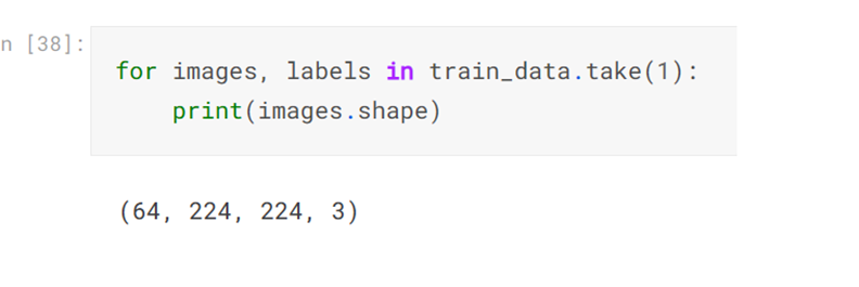
for images, labels in train_data.take(1):
    print(images.shape)
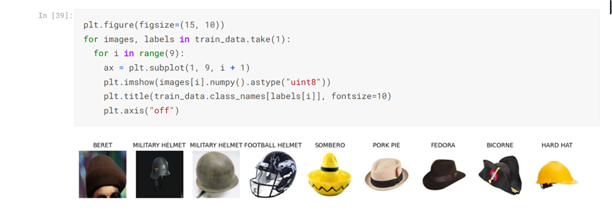
4. 探索数据
plt.figure(figsize=(15, 10))
for images, labels in train_data.take(1):
  for i in range(9):
    ax = plt.subplot(1, 9, i + 1)
    plt.imshow(images[i].numpy().astype("uint8"))
    plt.title(train_data.class_names[labels[i]], fontsize=10)
    plt.axis("off")
提取标签,如下行所示:
为train_data.class_names中的标签传递datal:中的每个标签
获取该标签文件夹中的文件名:OS . listdir(f " { data _ path }/{ label)")
获取文件名的计数:len().使用该标签名称和计数创建一个字典条目:label : len(
使用标签名称和计数创建字典条目:label : len(
label_counts = {label : len( os.listdir(f"{TRAINING_DIR}/{label}") ) for label in train_data.class_names }
NUM_CLASSES = len(label_counts)
 #将字典转换为熊猫系列以便于操作label_counts = pd。
label_counts = pd.Series(label_counts)
type(label_counts)
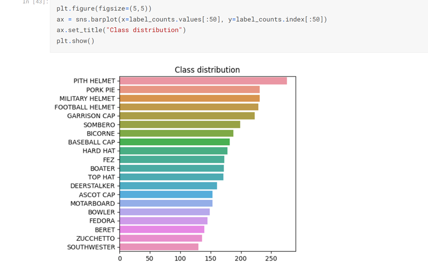
label_counts.sort_values(ascending=False, inplace=True)
plt.figure(figsize=(5,5))
ax = sns.barplot(x=label_counts.values[:50], y=label_counts.index[:50])
ax.set_title("Class distribution")
plt.show()
#少于150张图片的班级数量
label_counts[label_counts < 150]

# 从系列class _ NAMES = label _ counts . index . values CLASSES _ NAMES的第一列获取class _ NAMES
CLASSES_NAMES = label_counts.index.values
CLASSES_NAMES

5. 构建模型
由于我们有一个相对较小的数据集,其中有许多类,而且其中许多类只有很少的图像,因此,与从头开始训练模型相比,微调预训练模型将是一个更好的选择。让我们尝试一个ResNet58,看看它在我们的数据上的表现如何
预处理数据
使用Keras中ResNet50模型的函数preprocess_image_input对训练和验证集中的图像执行标准化。
def preprocess_image_input(image, label):
    image = tf.cast(image, tf.float32)
    image = tf.keras.applications.resnet50.preprocess_input(image)
    return image, label
train_data = train_data.map(preprocess_image_input)
val_data = val_data.map(preprocess_image_input)
定义网络
在Keras提供的ResNet50上执行迁移学习。
将预训练的imagenet权重加载到模型中。
选择保留ResNet50的所有层以及最终分类层。
'''
Feature Extraction is performed by ResNet50 pretrained on imagenet weights.
Input size is 224 x 224.
'''
def feature_extractor(inputs):

  feature_extractor = tf.keras.applications.resnet.ResNet50(input_shape=(224, 224, 3),
                                               include_top=False,
                                               weights='imagenet')(inputs)
  return feature_extractor
'''
Defines final dense layers and subsequent softmax layer for classification.
'''
def classifier(inputs):
    x = tf.keras.layers.GlobalAveragePooling2D()(inputs)
    x = tf.keras.layers.Flatten()(x)
    x = tf.keras.layers.Dense(1024, activation="relu")(x)
    x = tf.keras.layers.Dense(512, activation="relu")(x)
    x = tf.keras.layers.Dense(NUM_CLASSES, activation="softmax", name="classification")(x)
    return x
'''
Connect the feature extraction and "classifier" layers to build the model.
'''
def final_model(inputs):

    resize = tf.keras.layers.UpSampling2D(size=(7,7))(inputs)

    resnet_feature_extractor = feature_extractor(inputs)
    classification_output = classifier(resnet_feature_extractor)

    return classification_output
'''
Define the model and compile it.
Use Stochastic Gradient Descent as the optimizer.
Use Sparse Categorical CrossEntropy as the loss function.
'''
def define_compile_model():
  inputs = tf.keras.layers.Input(shape=(224,224,3))

  classification_output = final_model(inputs)
  model = tf.keras.Model(inputs=inputs, outputs = classification_output)

  model.compile(optimizer= tf.keras.optimizers.Adam(),
                loss='sparse_categorical_crossentropy',
                metrics = ['accuracy'])

  return model
model = define_compile_model()

model.summary()
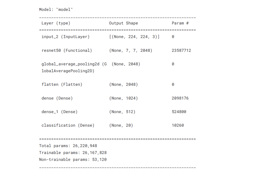
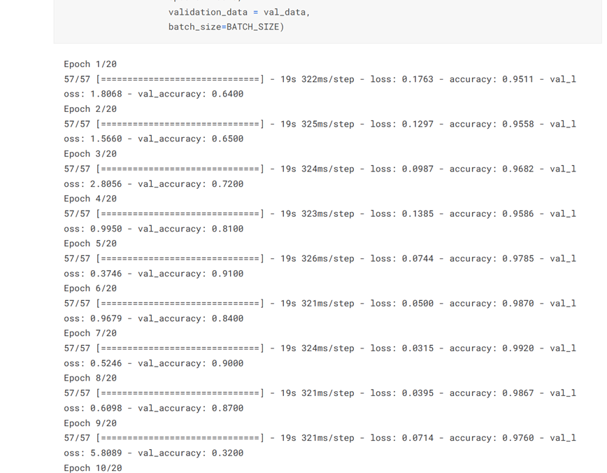
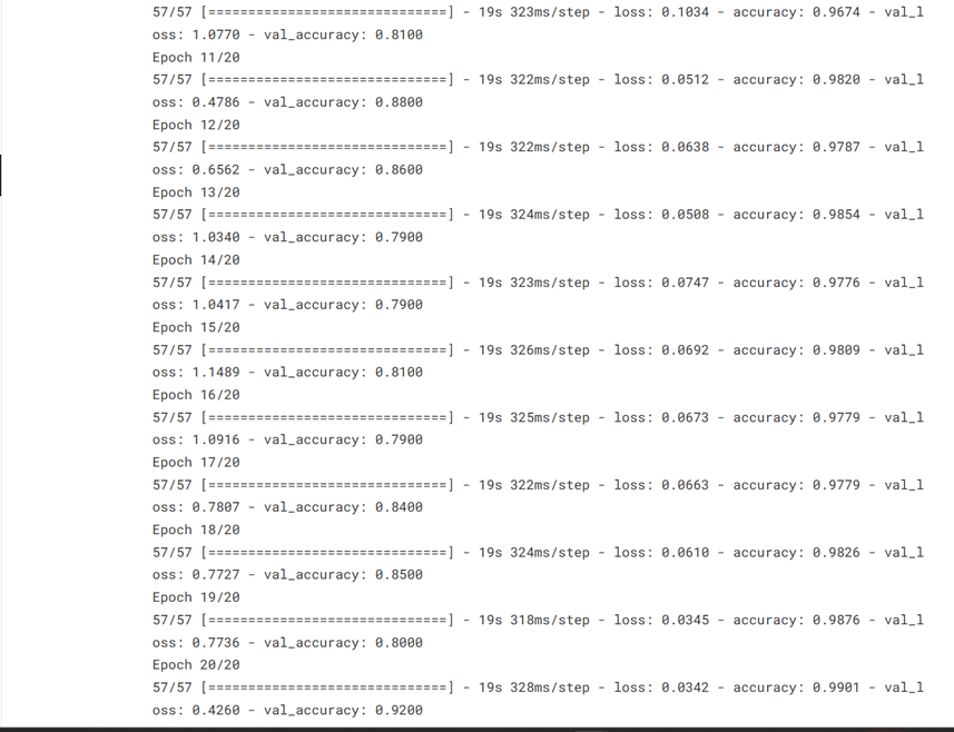
6. 训练模型
history = model.fit(train_data,
                    epochs=EPOCHS,
                    validation_data = val_data,
                    batch_size=BATCH_SIZE)
7定义一个函数来绘制训练数据
def tr_plot(tr_data):
    start_epoch=0
    #绘制训练和验证数据tacc=tr数据。
    tacc=tr_data.history['accuracy']
    tloss=tr_data.history['loss']
    vacc=tr_data.history['val_accuracy']
    vloss=tr_data.history['val_loss']
    tf1=tr_data.history['F1_score']
    vf1=tr_data.history['val_F1_score']
    Epoch_count=len(tacc)+ start_epoch
    Epochs=[]
    for i in range (start_epoch ,Epoch_count):
        Epochs.append(i+1)
index_loss=np.argmin(vloss) #这是具有最低验证损失的时期
    val_lowest=vloss[index_loss]
    index_acc=np.argmax(vacc)
    acc_highest=vacc[index_acc]
    indexf1=np.argmax(vf1)
    vf1_highest=vf1[indexf1]
    plt.style.use('fivethirtyeight')
    sc_label='best epoch= '+ str(index_loss+1 +start_epoch)
    vc_label='best epoch= '+ str(index_acc + 1+ start_epoch)
    f1_label='best epoch= '+ str(index_acc + 1+ start_epoch)
    fig,axes=plt.subplots(nrows=1, ncols=3, figsize=(25,10))
    axes[0].plot(Epochs,tloss, 'r', label='Training loss')
    axes[0].plot(Epochs,vloss,'g',label='Validation loss' )
    axes[0].scatter(index_loss+1 +start_epoch,val_lowest, s=150, c= 'blue', label=sc_label)
    axes[0].scatter(Epochs, tloss, s=100, c='red')
    axes[0].set_title('Training and Validation Loss')
    axes[0].set_xlabel('Epochs', fontsize=18)
    axes[0].set_ylabel('Loss', fontsize=18)
    axes[0].legend()
    axes[1].plot (Epochs,tacc,'r',label= 'Training Accuracy')
    axes[1].scatter(Epochs, tacc, s=100, c='red')
    axes[1].plot (Epochs,vacc,'g',label= 'Validation Accuracy')
    axes[1].scatter(index_acc+1 +start_epoch,acc_highest, s=150, c= 'blue', label=vc_label)
    axes[1].set_title('Training and Validation Accuracy')
    axes[1].set_xlabel('Epochs', fontsize=18)
    axes[1].set_ylabel('Accuracy', fontsize=18)
    axes[1].legend()
    axes[2].plot (Epochs,tf1,'r',label= 'Training F1 score')
    axes[2].plot (Epochs,vf1,'g',label= 'Validation F1 score')
index_tf1=np.argmax(tf1) #这是tr最高的epoch
    tf1max=tf1[index_tf1]
    index_vf1=np.argmax(vf1) #这是f1得分最高的时期
    vf1max=vf1[index_vf1]
    axes[2].scatter(index_vf1+1 +start_epoch,vf1max, s=150, c= 'blue', label=vc_label)
    axes[2].scatter(Epochs, tf1, s=100, c='red')
    axes[2].set_title('Training and Validation F1 score')
    axes[2].set_xlabel('Epochs', fontsize=18)
    axes[2].set_ylabel('F1  score', fontsize=18)
    axes[2].legend()
    plt.tight_layout
    plt.show()
    return
定义一个函数以将训练数据保存到
def save_history_to_csv(history,csvpath):
    trdict=history.history
    df=pd.DataFrame()
    df['Epoch']=list(np.arange(1, len(trdict['loss']) + 1 ))
    keys=list(trdict.keys())
    for key in keys:
        data=list(trdict[key])
        df[key]=data
    df.to_csv(csvpath, index=False)
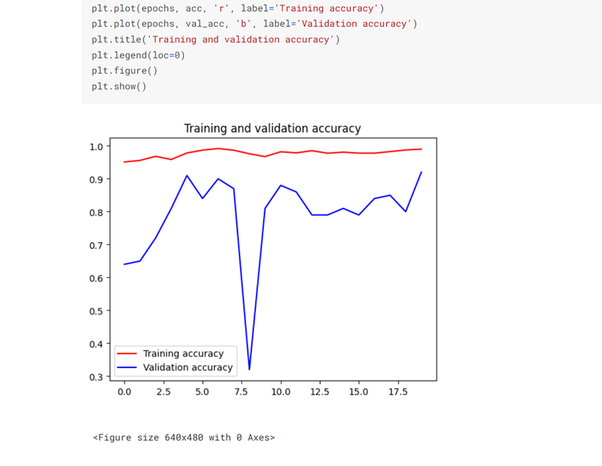
8. 绘制损失和精度曲线
import matplotlib.pyplot as plt
acc = history.history['accuracy']
val_acc = history.history['val_accuracy']

epochs = range(len(acc))

plt.plot(epochs, acc, 'r', label='Training accuracy')
plt.plot(epochs, val_acc, 'b', label='Validation accuracy')
plt.title('Training and validation accuracy')
plt.legend(loc=0)
plt.figure()
plt.show()
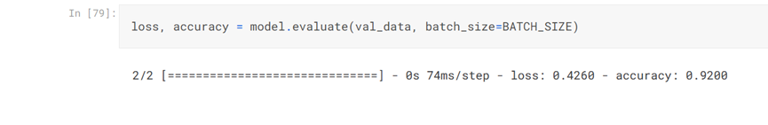
9. 评估模型
使用模型的计算损失和准确性指标。
loss, accuracy = model.evaluate(val_data, batch_size=BATCH_SIZE)
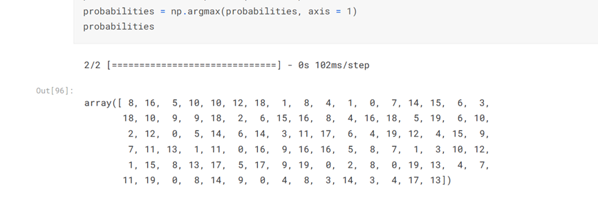
10. 测试模型
 #获取图像的预测概率概率= model.predict(test_data)
probabilities = model.predict(test_data)
probabilities = np.argmax(probabilities, axis = 1)
probabilities
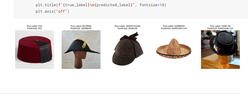
plt.figure(figsize=(20, 10))
for images, labels in test_data.take(1):
    for i in range(5):
        ax = plt.subplot(1, 5, i + 1)
        plt.imshow(images[i].numpy().astype("uint8"))
        #获取真实标签和预测的类名
        true_label = 'True Label: '+test_data.class_names[labels[i]]
        predicted_label = 'Predicted: '+test_data.class_names[probabilities[i]]
      #设置子情节的标题
        plt.title(f"{true_label}\n{predicted_label}", fontsize=10)
        plt.axis("off")
  1 try:
  2   # %tensorflow_version 仅存在于Colab中
  3   %tensorflow_version 2.x
  4 except Exception:
  5   pass
  6
  7 import warnings
  8 warnings.filterwarnings('ignore')
  9
 10
 11 import os, re, time, json
 12 import PIL.Image, PIL.ImageFont, PIL.ImageDraw
 13 import numpy as np
 14 import pandas as pd
 15
 16 import tensorflow as tf
 17 from tensorflow import keras
 18 from tensorflow.keras.utils import image_dataset_from_directory
 19 from tensorflow.keras.applications.resnet50 import ResNet50
 20 from matplotlib import pyplot as plt
 21 import tensorflow_datasets as tfds
 22
 23 import matplotlib.pyplot as plt
 24 import seaborn as sns
 25
 26 print("Tensorflow version " + tf.__version__)
 27
 28 #常量
 29 SPLIT_SIZE = .2
 30 BATCH_SIZE = 64
 31 IMG_SIZE = (224, 224)
 32 EPOCHS=20
 33
 34 # 创建一些文件夹来存储培训和测试数据
 35
 36 TRAINING_DIR ="/tm/input/headgear-image-classification/train/"
 37 Valid_DIR="/tm/input/headgear-image-classification/valid/"
 38 TESTING_DIR ="/tm/input/headgear-image-classification/test/"
 39
 40 train_data = image_dataset_from_directory(TRAINING_DIR,
 41                                           batch_size=BATCH_SIZE,
 42                                           image_size=IMG_SIZE
 43                                          )
 44
 45 val_data = image_dataset_from_directory(Valid_DIR,
 46                                         batch_size=BATCH_SIZE,
 47                                         image_size=IMG_SIZE
 48                                        )
 49
 50 test_data = image_dataset_from_directory(TESTING_DIR,
 51                                          batch_size=BATCH_SIZE,
 52                                          image_size=IMG_SIZE
 53                                         )
 54
 55 for images, labels in train_data.take(1):
 56     print(images.shape)
 57
 58 plt.figure(figsize=(15, 10))
 59 for images, labels in train_data.take(1):
 60   for i in range(9):
 61     ax = plt.subplot(1, 9, i + 1)
 62     plt.imshow(images[i].numpy().astype("uint8"))
 63     plt.title(train_data.class_names[labels[i]], fontsize=10)
 64     plt.axis("off")
 65
 66 label_counts = {label : len( os.listdir(f"{TRAINING_DIR}/{label}") ) for label in train_data.class_names }
 67 NUM_CLASSES = len(label_counts)
 68
 69 #将字典转换为熊猫系列以便于操作label_counts = pd。
 70 label_counts = pd.Series(label_counts)
 71 type(label_counts)
 72
 73 label_counts.sort_values(ascending=False, inplace=True)
 74
 75 plt.figure(figsize=(5,5))
 76 ax = sns.barplot(x=label_counts.values[:50], y=label_counts.index[:50])
 77 ax.set_title("Class distribution")
 78 plt.show()
 79
 80 #少于150张图片的班级数量
 81 label_counts[label_counts < 150]
 82
 83 # 从系列class _ NAMES = label _ counts . index . values CLASSES _ NAMES的第一列获取class _ NAMES
 84 CLASSES_NAMES = label_counts.index.values
 85 CLASSES_NAMES
 86
 87 def preprocess_image_input(image, label):
 88     image = tf.cast(image, tf.float32)
 89     image = tf.keras.applications.resnet50.preprocess_input(image)
 90     return image, label
 91
 92 train_data = train_data.map(preprocess_image_input)
 93 val_data = val_data.map(preprocess_image_input)
 94
 95 '''
 96 Feature Extraction is performed by ResNet50 pretrained on imagenet weights.
 97 Input size is 224 x 224.
 98 '''
 99 def feature_extractor(inputs):
100
101   feature_extractor = tf.keras.applications.resnet.ResNet50(input_shape=(224, 224, 3),
102                                                include_top=False,
103                                                weights='imagenet')(inputs)
104   return feature_extractor
105
106 '''
107 Defines final dense layers and subsequent softmax layer for classification.
108 '''
109 def classifier(inputs):
110     x = tf.keras.layers.GlobalAveragePooling2D()(inputs)
111     x = tf.keras.layers.Flatten()(x)
112     x = tf.keras.layers.Dense(1024, activation="relu")(x)
113     x = tf.keras.layers.Dense(512, activation="relu")(x)
114     x = tf.keras.layers.Dense(NUM_CLASSES, activation="softmax", name="classification")(x)
115     return x
116
117 '''
118 Connect the feature extraction and "classifier" layers to build the model.
119 '''
120 def final_model(inputs):
121
122     resize = tf.keras.layers.UpSampling2D(size=(7,7))(inputs)
123
124     resnet_feature_extractor = feature_extractor(inputs)
125     classification_output = classifier(resnet_feature_extractor)
126
127     return classification_output
128
129 '''
130 Define the model and compile it.
131 Use Stochastic Gradient Descent as the optimizer.
132 Use Sparse Categorical CrossEntropy as the loss function.
133 '''
134 def define_compile_model():
135   inputs = tf.keras.layers.Input(shape=(224,224,3))
136
137   classification_output = final_model(inputs)
138   model = tf.keras.Model(inputs=inputs, outputs = classification_output)
139
140   model.compile(optimizer= tf.keras.optimizers.Adam(),
141                 loss='sparse_categorical_crossentropy',
142                 metrics = ['accuracy'])
143
144   return model
145
146 model = define_compile_model()
147
148 model.summary()
149
150 history = model.fit(train_data,
151                     epochs=EPOCHS,
152                     validation_data = val_data,
153                     batch_size=BATCH_SIZE)
154
155 def tr_plot(tr_data):
156     start_epoch=0
157 #绘制训练和验证数据tacc=tr数据。
158 tacc=tr_data.history['accuracy']
159     tloss=tr_data.history['loss']
160     vacc=tr_data.history['val_accuracy']
161     vloss=tr_data.history['val_loss']
162     tf1=tr_data.history['F1_score']
163     vf1=tr_data.history['val_F1_score']
164     Epoch_count=len(tacc)+ start_epoch
165     Epochs=[]
166     for i in range (start_epoch ,Epoch_count):
167         Epochs.append(i+1)
168 index_loss=np.argmin(vloss) #这是具有最低验证损失的时期
169 val_lowest=vloss[index_loss]
170     index_acc=np.argmax(vacc)
171     acc_highest=vacc[index_acc]
172     indexf1=np.argmax(vf1)
173     vf1_highest=vf1[indexf1]
174     plt.style.use('fivethirtyeight')
175     sc_label='best epoch= '+ str(index_loss+1 +start_epoch)
176     vc_label='best epoch= '+ str(index_acc + 1+ start_epoch)
177     f1_label='best epoch= '+ str(index_acc + 1+ start_epoch)
178     fig,axes=plt.subplots(nrows=1, ncols=3, figsize=(25,10))
179     axes[0].plot(Epochs,tloss, 'r', label='Training loss')
180     axes[0].plot(Epochs,vloss,'g',label='Validation loss' )
181     axes[0].scatter(index_loss+1 +start_epoch,val_lowest, s=150, c= 'blue', label=sc_label)
182     axes[0].scatter(Epochs, tloss, s=100, c='red')
183     axes[0].set_title('Training and Validation Loss')
184     axes[0].set_xlabel('Epochs', fontsize=18)
185     axes[0].set_ylabel('Loss', fontsize=18)
186     axes[0].legend()
187     axes[1].plot (Epochs,tacc,'r',label= 'Training Accuracy')
188     axes[1].scatter(Epochs, tacc, s=100, c='red')
189     axes[1].plot (Epochs,vacc,'g',label= 'Validation Accuracy')
190     axes[1].scatter(index_acc+1 +start_epoch,acc_highest, s=150, c= 'blue', label=vc_label)
191     axes[1].set_title('Training and Validation Accuracy')
192     axes[1].set_xlabel('Epochs', fontsize=18)
193     axes[1].set_ylabel('Accuracy', fontsize=18)
194     axes[1].legend()
195     axes[2].plot (Epochs,tf1,'r',label= 'Training F1 score')
196     axes[2].plot (Epochs,vf1,'g',label= 'Validation F1 score')
197 index_tf1=np.argmax(tf1) #这是tr最高的epoch
198     tf1max=tf1[index_tf1]
199 index_vf1=np.argmax(vf1) #这是f1得分最高的时期
200     vf1max=vf1[index_vf1]
201     axes[2].scatter(index_vf1+1 +start_epoch,vf1max, s=150, c= 'blue', label=vc_label)
202     axes[2].scatter(Epochs, tf1, s=100, c='red')
203     axes[2].set_title('Training and Validation F1 score')
204     axes[2].set_xlabel('Epochs', fontsize=18)
205     axes[2].set_ylabel('F1  score', fontsize=18)
206     axes[2].legend()
207     plt.tight_layout
208     plt.show()
209     return
210
211 def save_history_to_csv(history,csvpath):
212     trdict=history.history
213     df=pd.DataFrame()
214     df['Epoch']=list(np.arange(1, len(trdict['loss']) + 1 ))
215     keys=list(trdict.keys())
216     for key in keys:
217         data=list(trdict[key])
218         df[key]=data
219     df.to_csv(csvpath, index=False)
220
221 import matplotlib.pyplot as plt
222 acc = history.history['accuracy']
223 val_acc = history.history['val_accuracy']
224
225 epochs = range(len(acc))
226
227 plt.plot(epochs, acc, 'r', label='Training accuracy')
228 plt.plot(epochs, val_acc, 'b', label='Validation accuracy')
229 plt.title('Training and validation accuracy')
230 plt.legend(loc=0)
231 plt.figure()
232 plt.show()
233
234 loss, accuracy = model.evaluate(val_data, batch_size=BATCH_SIZE)
235
236 # 获取图像的预测概率概率= model.predict(test_data)
237 probabilities = model.predict(test_data)
238 probabilities = np.argmax(probabilities, axis = 1)
239 probabilities
240
241 plt.figure(figsize=(20, 10))
242 for images, labels in test_data.take(1):
243     for i in range(5):
244         ax = plt.subplot(1, 5, i + 1)
245         plt.imshow(images[i].numpy().astype("uint8"))
246          #获取真实标签和预测的类名
247         true_label = 'True Label: '+test_data.class_names[labels[i]]
248         predicted_label = 'Predicted: '+test_data.class_names[probabilities[i]]
249       #设置子情节的标题
250         plt.title(f"{true_label}\n{predicted_label}", fontsize=10)
251         plt.axis("off")