概
自监督加图用于 session 推荐, 还用到了对抗训练, 只能说作者 coding 能力是一流的.
符号说明
- \(I = \{i_1, i_2, i_3, \ldots, i_N\}\), items;
- \(s = [i_{s,1}, i_{s, 2}, i_{s, 3}, \ldots, i_{s, m}]\), 某个 session 序列;
- \(\mathbf{X}^{(l)} \in \mathbb{R}^{N \times d^{(l)}}\) 表示神经网络第 \(l\) 层的 embeddings, \(\mathbf{X}^{(0)}\) 为初始的 embeddings;
- \(y = [y_1, y_2, y_3, \ldots, y_N]\) 为 ranked list;
COTREC
图的构建
-
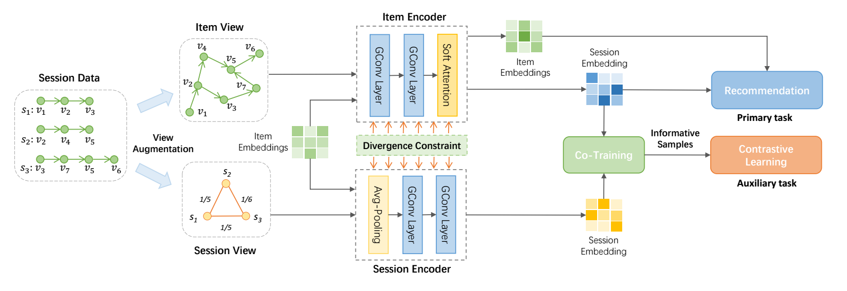
如上图所示, 我们需要构建 item-item 图和 session-session 图.
-
item-item 图中两个结点存在边当二者在某个 session 中为前后关系, 记 item-item 图的邻接矩阵为 \(\mathbf{A}_I\), 则
\[\mathbf{A}_{I,i,j} = |\{(s, k): \exist k, \: s_k = v_i, s_{k+1} = v_j\}|. \] -
而 session-session 图中, 两个 session 存在边当二者存在相同的结点, 记 session-session 图的邻接矩阵为 \(\mathbf{A}_S\), 则
\[\mathbf{A}_{S, p, q} = \frac{|s_p \cap s_q|}{|s_p \cup s_q|}. \]
Item View Encoding
-
Item view encoding 首先需要经过一系列的图卷积, 每一层如下:
\[\mathbf{X}_I^{(l+1)} = \mathbf{\hat{D}}_I^{-1} \mathbf{\hat{A}}_{I} \mathbf{X}_I^{(l)} \mathbf{W}_I^l, \]其中 \(\mathbf{\hat{A}}_I = \mathbf{A}_I + \mathbf{I}\), \(\mathbf{\hat{D}}_I\) 为对应的 degree matrix.
-
经过 \(L\) 层后, 综合各层的结果 (就像 LightGCN 一样):
\[\mathbf{X}_I = \frac{1}{L + 1} \sum_{l=0}^L \mathbf{X}_I^{(l)}. \] -
然后, 作者模范 GCE-GNN 的思路, 引入可学习的位置编码 (针对 session 序列 \(s = [i_{s,1}, i_{s, 2}, i_{s, 3}, \ldots, i_{s, m}]\)):
\[\mathbf{P}_r = [\mathbf{p}_1, \mathbf{p}_2, \mathbf{p}_3, \ldots, \mathbf{p}_m], \]然后:
\[\mathbf{x}_I^{t*} = \tanh (\mathbf{W}_1[\mathbf{x}_I^t \| \mathbf{p}_{m-t+1}] + \mathbf{b}), \]其中 \(\mathbf{W}_1 \in \mathbb{R}^{d \times 2d}, \mathbf{b} \in \mathbb{R}^d\) 为可训练的参数. 注意, 这里位置编码是倒序的, 以保证各位置的重要性不受序列长度的影响. \(\mathbf{x}_I^t\) 为序列 \(s\) 中第 \(t\) 个位置对应的 embedding.
-
最后, 通过 soft-attention 机制将 session 中的各 item 进行融合:
\[\theta_I = \sum_{t=1}^m \alpha \mathbf{x}_I^{t*}, \\ \alpha_t = \mathbf{f}^T \sigma(\mathbf{W}_2 \mathbf{x}_s + \mathbf{W}_3 \mathbf{x}_I^{t*} + \mathbf{c}), \\ \mathbf{x}_s = \frac{1}{m} \sum_{t=1}^m \mathbf{x}_I^m \]
Session View Encoding
-
首先, 初始 session 序列的 embeddings 为
\[[\Theta_S^{(0)}]_s = \sum_{i \in s} \mathbf{x}_i^{(0)}. \] -
然后经过图卷积得到:
\[\Theta_S^{(l+1)} = \mathbf{\hat{D}}_S^{-1} \mathbf{\hat{A}}_S \Theta_S^{(l)} \mathbf{W}_S^{(l)}, \]其中的符号和之前的定义是类似的.
-
之后, 依旧采用平均的方式融合各层的结果:
\[\Theta_S = \frac{1}{L+1} \sum_{l=0}^L \Theta_S^{(l)}. \]
Co-Training
-
现在, 我们得到了两个 view 的 session 特征表示 \(\theta_I, \Theta_S\), 以及 item 的表示 \(\mathbf{X}^{(0)}, \mathbf{X}_I\).
-
我们希望利用 co-training 互补地得到伪标签.
-
首先, 利用 item-view 得到 session \(p\) 对各 items 的 score:
\[\mathbf{y}_I^{p} = \text{Softmax}(\mathbf{X}_I \theta_I^p). \] -
其次, 利用 session-view 得到 session \(p\) 对各 items 的 score:
\[\mathbf{y}_S^{p} = \text{Softmax}(\mathbf{X}^{(0)} \theta_S^p). \]这里我们使用 \(\mathbf{X}^{(0)}\) 的原因是, session-view 这一侧并没有像 item-view 一样输出 \(\mathbf{X}_I\).
-
接着, 我们将:
\[c_S^{p^+} = \text{top-K}(\mathbf{y}_I^{p}) \]作为 session-view 的正样本, 另外
\[c_S^{p^-} = \text{top-10\%}(\mathbf{y}_I^{p}) \setminus c_S^{p_+} \]作为负样本. 对于 item-view 的正样本和负样本可以类似得到.
Contrastive Learning
-
我们利用对比学习和上面的正负样本进行训练:
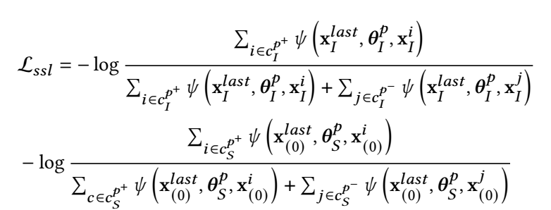
其中 \(\mathbf{x}^{last}\) 是 last-clicked item, \(\psi(\mathbf{x}_1, \mathbf{x}_2, \mathbf{x}_3) = \exp(f(\mathbf{x}_1 + \mathbf{x}_2, \mathbf{x}_3 + \mathbf{x}_2) / \tau)\), 其中 \(f: \mathbb{R}^d \times \mathbb{R}^d \rightarrow \mathbb{R}\) 建模两个向量的 agreement, 作者实际用 cosine, 和一般的对比学习是一致的. -
简而言之, 作者希望最后一个 item + 综合的信息 和 正样本 + 综合的信息 之间要尽可能相近, 而 item + 综合的信息 和 负样本 + 综合的信息 要尽可能远离.
Divergence Constraint
-
为了防止两个 encoder 输出过于相似的特征, 作者引入 divergence constraint.
-
要求:
\[\mathcal{L}_{\text{diff}} = \text{KL}(Prob_I(\mathbf{X}_I), Prob_S(\mathbf{X}_I + \Delta_{adv}^I)) + \text{KL}(Prob_S(\mathbf{X}_I), Prob_I(\mathbf{I} + \Delta_{adv}^S)). \]其中 \(Prob_I(\mathbf{X}_I) = \text{Softmax}(\mathbf{X}_I\theta_I^{p}), Prob_S(\mathbf{X}_I) = \text{Softmax}(\mathbf{X}_I\theta_S^p)\). 这里的 \(\Delta\) 是通过 FGSM 构造的.
优化
-
除了上面的对比损失和 \(\mathcal{L}_{\text{diff}}\) 外, 我们再引入一般的推荐损失:
\[\mathcal{L}_r = -\sum_{i=1}^N \mathbf{y}_i \log (\mathbf{\hat{y}}_i) + (1 - \mathbf{y}_i) \log (1 - \mathbf{\hat{y}}_i), \\ \mathbf{\hat{y}} = \text{Softmax}(\mathbf{\hat{z}}), \\ \mathbf{\hat{z}}_i = {\theta_I^s}^T \mathbf{x}_i. \]这里作者将 item-view 作者为主 encoder.
-
最后的损失为:
\[\mathcal{L} = \mathcal{L}_r + \beta \mathcal{L}_{ssl} + \alpha \mathcal{L}_{\text{diff}}. \]
代码
- Self-Supervised Recommendation Session-based Co-Training Supervisedself-supervised recommendation session-based self-supervised recommendation convolutional self-supervised recommendation session-based information exploiting recommendation session-based information handling self-supervised exploration generative supervised self-supervised transformers lightweight supervised self-supervised interpretable adversarial generative recommendation session-based priority session self-supervised transformers supervised empirical