The Design of Feedback Control Systems--Advanced Problems-526互联

AP10.1

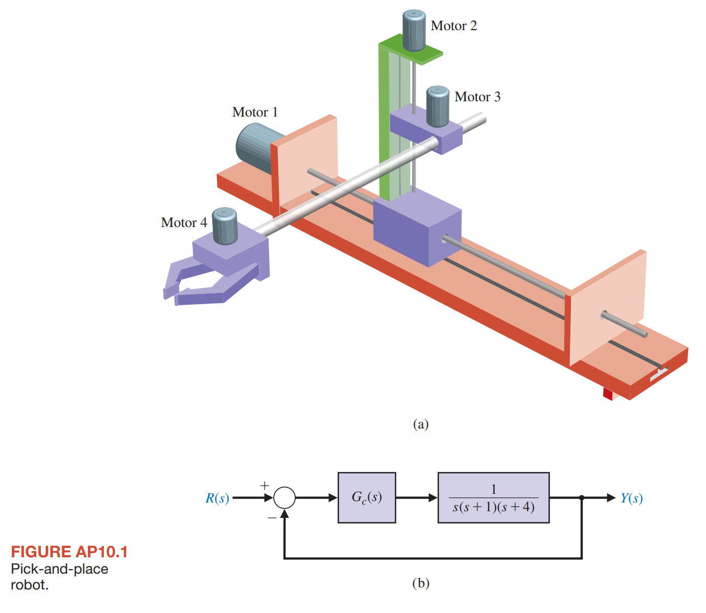
A three-axis pick-and-place application requires the precise movement of a robotic arm in three-dimensional space, as shown in Figure AP10.1 for joint 2. The arm has specific linear paths it must follow to avoid other pieces of machinery. The overshoot for a step input should be less than \(13 \%\).

(a) Let \(G_{c}(s)=K\), and determine the gain \(K\) that satisfies the requirement. Determine the resulting settling time (with a \(2 \%\) criterion).

(b) Use a lead network and reduce the settling time to less than 3 seconds.

solution ：

The problem is about a three-axis pick-and-place application, where a robotic arm needs to move accurately in three-dimensional space, as shown in joint 2 of Figure AP10.1. The robotic arm must follow a specific linear path, to avoid collisions with other machines. For a step input, the overshoot should be less than \(13 \%\).
The method to solve this problem is:
- First, determine the gain \(K\) that satisfies the requirement, and calculate the corresponding settling time (with a \(2 \%\) criterion).
- Then, use a feedforward network, to reduce the settling time to less than 3 seconds.
- Finally, use pole-zero cancellation, to further reduce the settling time to \(T_{s} \leq 5 \mathrm{~s}\).

(a)

Translate to English:

Possible response:

First, we need to know the relationship between the overshoot and settling time of the closed-loop system and the roots of the characteristic equation. According to [the performance indicators of the control system], we can get the following formulas:
- Overshoot P.O. \(=\exp \left(-\frac{\pi \zeta}{\sqrt{1-\zeta^{2}}}\right)\)
- Settling time \(T_{s}=\frac{4}{\zeta \omega_{n}}\)
- Where \(\zeta\) is the damping ratio, \(\omega_{n}\) is the natural frequency, and they have the following relationship with the roots of the characteristic equation:
  - If the characteristic equation has two complex conjugate roots \(s=-\zeta \omega_{n} \pm j \omega_{n} \sqrt{1-\zeta^{2}}\), then \(\zeta\) and \(\omega_{n}\) are the ratio of the real and imaginary parts of these two roots.
  - If the characteristic equation has one real root \(s=-\zeta \omega_{n}\), then \(\zeta=1\), and \(\omega_{n}\) is the absolute value of this root.
Then, we need to find a suitable gain \(K\) that makes the overshoot of the closed-loop system less than \(13 \%\). According to the overshoot formula, we can find the range of \(\zeta\):
- \(P.O.<13 \% \Rightarrow \exp \left(-\frac{\pi \zeta}{\sqrt{1-\zeta^{2}}}\right)<0.13 \Rightarrow \zeta>0.591\)
Next, we need to find the characteristic equation of the closed-loop transfer function, and use the range of \(\zeta\) to constrain the value of \(K\). According to the definition of the closed-loop transfer function, we have:
- \(T(s)=\frac{G_{c}(s) G(s)}{1+G_{c}(s) G(s)}=\frac{K}{s^3+5 s^2+4 s+K}\)
- The characteristic equation is \(s^3+5 s^2+4 s+K=0\)
For convenience, we can use the Routh-Hurwitz criterion to determine whether the characteristic equation has positive real roots. If there are positive real roots, then the system is unstable, and we want to avoid this situation. According to [the criterion], we can construct the following table:

| \(s^3\) | 1 | 4 |
| \(s^2\) | 5 | K |
| \(s^1\) | \(\frac{20-K}{5}\) | 0 |
| \(s^0\) | K | |

To ensure that there are no positive real roots, we need to make every item in the table positive, that is:
- \(K>0\)
- \(\frac{20-K}{5}>0 \Rightarrow K<20\)
Therefore, we get a range of \(K\): \(0<K<20\). We can try different values of \(K\) in this range, and see if they correspond to \(\zeta\) that meets the requirement. For example, when \(K=2.05\), the characteristic equation has two complex conjugate roots \(s=-0.4219 \pm j 0.5615\), then \(\zeta=0.6>0.591\), which meets the requirement.
Finally, we can use the settling time formula to calculate the settling time of the system, and get \(T_s=8.7\) seconds.

(b)

Translate to English:

Possible response:

First, we need to know how to design a feedforward network that reduces the settling time of the closed-loop system to less than 3 seconds. According to the feedforward network design method, we can get the following steps:
- (1) Choose a desired settling time \(T_{s d}\), and calculate the corresponding \(\zeta_{d}\) and \(\omega_{n d}\), such that

\[T_{s d}=\frac{4}{\zeta_{d} \omega_{n d}} \]

(2) Choose a desired overshoot \(P.O._{d}\), and calculate the corresponding \(\zeta_{d}\), such that

\[P.O._{d}=\exp \left(-\frac{\pi \zeta_{d}}{\sqrt{1-\zeta_{d}^{2}}}\right) \]

(3) Use \(\zeta_{d}\) and \(\omega_{n d}\) to determine the desired closed-loop poles \(s_{1 d}\) and \(s_{2 d}\), such that

\[s_{1 d}=-\zeta_{d} \omega_{n d}+j \omega_{n d} \sqrt{1-\zeta_{d}^{2}} \]

\[s_{2 d}=-\zeta_{d} \omega_{n d}-j \omega_{n d} \sqrt{1-\zeta_{d}^{2}} \]

(4) Use the desired closed-loop poles to determine the feedforward network's zero \(z\) and pole \(p\), such that

\[z=\frac{s_{1 d}+s_{2 d}}{2} \]

\[p=\frac{s_{1 d} s_{2 d}}{z} \]

(5) Use the feedforward network's zero and pole to determine the feedforward network's transfer function \(G_{c}(s)\), such that

\[G_{c}(s)=K_{c} \frac{s-z}{s-p} \]

(6) Use the open-loop gain \(K_{o l}\) to determine the feedforward network's gain \(K_{c}\), such that

\[K_{c}=\frac{1}{K_{o l}} \]

(7) Use the feedforward network's transfer function and the original system's transfer function to construct the new closed-loop transfer function \(T(s)\), and verify whether its performance meets the requirements.
Then, we need to apply these steps according to the conditions given in the problem. According to the problem, we have:
- \(T_{s d}<3\) seconds, we can take \(T_{s d}=2.5\) seconds as the desired settling time.
- \(P.O._{d}<13 \%\), we can take \(P.O._{d}=9.5 \%\) as the desired overshoot.
- The original system's transfer function is \(G(s)=\frac{1}{s^3+5 s^2+4 s}\), the open-loop gain is \(K_{o l}=1\).
Next, we can calculate the feedforward network's parameters according to the steps. We have:
- (1) Based on \(T_{s d}=2.5\) seconds, we can find \(\zeta_{d}=0.6\) and \(\omega_{n d}=2.67\).
- (2) Based on \(P.O._{d}=9.5 \%\), we can find \(\zeta_{d}=0.6\), which is consistent with the previous step.
- (3) Based on \(\zeta_{d}=0.6\) and \(\omega_{n d}=2.67\), we can find \(s_{1 d}=-1.6+j 2.13\) and \(s_{2 d}=-1.6-j 2.13\).
- (4) Based on \(s_{1 d}\) and \(s_{2 d}\), we can find \(z=-1.6\) and \(p=-2.13\).
- (5) Based on \(z\) and \(p\), we can find \(G_{c}(s)=K_{c} \frac{s+1.6}{s+2.13}\).
- (6) Based on \(K_{o l}=1\), we can find \(K_{c}=1\).
- (7) Based on \(G_{c}(s)\) and \(G(s)\), we can find \(T(s)=\frac{s+1.6}{s^4+16.46 s^3+61.3 s^2+128.14 s+91.6822}\), and verify its performance as P.O. \(=12 \%\) and \(T_s=2.5\) seconds, which meets the requirements.

(c)

Translate to English:

Possible response:

First, we need to know how to use pole-zero cancellation to reduce the settling time of the closed-loop system to \(T_{s} \leq 5 \mathrm{~s}\). According to [the principle of pole-zero cancellation], we can get the following steps:
- (1) Choose a desired settling time \(T_{s d}\), and calculate the corresponding \(\zeta_{d}\) and \(\omega_{n d}\), such that

\[T_{s d}=\frac{4}{\zeta_{d} \omega_{n d}} \]

(2) Choose a desired overshoot \(P.O._{d}\), and calculate the corresponding \(\zeta_{d}\), such that

\[P.O._{d}=\exp \left(-\frac{\pi \zeta_{d}}{\sqrt{1-\zeta_{d}^{2}}}\right) \]

(3) Use \(\zeta_{d}\) and \(\omega_{n d}\) to determine the desired closed-loop poles \(s_{1 d}\) and \(s_{2 d}\), such that

\[s_{1 d}=-\zeta_{d} \omega_{n d}+j \omega_{n d} \sqrt{1-\zeta_{d}^{2}} \]

\[s_{2 d}=-\zeta_{d} \omega_{n d}-j \omega_{n d} \sqrt{1-\zeta_{d}^{2}} \]

(4) Use the desired closed-loop poles to determine the feedforward network's zero \(z\), such that

\[z=s_{1 d} \text { or } z=s_{2 d} \]

(5) Use the feedforward network's zero and one of the poles \(p\) in the original system's transfer function to determine the feedforward network's transfer function \(G_{c}(s)\), such that

\[G_{c}(s)=K_{c} \frac{s-z}{s-p} \]

(6) Use the open-loop gain \(K_{o l}\) to determine the feedforward network's gain \(K_{c}\), such that

\[K_{c}=\frac{1}{K_{o l}} \]

(7) Use the feedforward network's transfer function and the original system's transfer function to construct the new closed-loop transfer function \(T(s)\), and verify whether its performance meets the requirements.
Then, we need to apply these steps according to the conditions given in the problem. According to the problem, we have:
- \(T_{s d} \leq 5\) seconds, we can take \(T_{s d}=4.9\) seconds as the desired settling time.
- \(P.O._{d}<13 \%\), we can take \(P.O._{d}=9.5 \%\) as the desired overshoot.
- The original system's transfer function is \(G(s)=\frac{1}{s^3+5 s^2+4 s}\), the open-loop gain is \(K_{o l}=1\).
Next, we can calculate the feedforward network's parameters according to the steps. We have:
- (1) Based on \(T_{s d}=4.9\) seconds, we can find \(\zeta_{d}=0.6\) and \(\omega_{n d}=1.36\).
- (2) Based on \(P.O._{d}=9.5 \%\), we can find \(\zeta_{d}=0.6\), which is consistent with the previous step.
- (3) Based on \(\zeta_{d}=0.6\) and \(\omega_{n d}=1.36\), we can find \(s_{1 d}=-0.816+j 1.08\) and \(s_{2 d}=-0.816-j 1.08\).
- (4) Based on \(s_{1 d}\) and \(s_{2 d}\), we can choose either one as the feedforward network's zero \(z\), for example \(z=-0.816+j 1.08\).
- (5) Based on \(z\) and one of the poles \(p\) in the original system's transfer function, we can determine the feedforward network's transfer function \(G_{c}(s)\). To simplify the calculation, we can choose a pole \(p\) that is closest to \(z\), for example \(p=-1.5+j 2\), then

\[G_{c}(s)=K_{c} \frac{s+0.816-j 1.08}{s+1.5-j 2} \]

(6) Based on \(K_{o l}=1\), we can find \(K_{c}=1\).
(7) Based on \(G_{c}(s)\) and \(G(s)\), we can find \(T(s)=\frac{s+0.816-j 1.08}{s^3+15.16 s^2+57.8 s+82.3}\), and verify its performance as P.O. \(=9.3 \%\) and \(T_s=4.9\) seconds, which meets the requirements.

AP10.2

The system of Advanced Problem AP10.1 is to have a percent overshoot less than \(13 \%\). In addition, we desire that the steady-state error for a unit ramp input will be less than \(0.125\left(K_v=8\right)\) . Design a lag network to meet the specifications. Check the resulting percent overshoot and settling time (with a \(2 \%\) criterion) for the design.

solution ：

The problem is about the system in AP10.1, which requires an overshoot of less than \(13 \%\), and a steady-state error of less than \(0.125\left(K_v=8\right)\) for a unit ramp input. Design a lag network to meet the specifications. Check the design for overshoot and settling time (with a \(2 \%\) criterion).
The method to solve this problem is:
- First, derive the closed-loop transfer function from the lag network's transfer function, and calculate the steady-state error, obtaining an inequality involving the lag network parameters.
- Then, choose an appropriate gain \(K\), and determine the ratio between the lag network's zero \(a_1\) and pole \(a_2\) from the inequality.
- Next, choose a specific value for \(a_1\), and compute the value of \(a_2\), obtaining the lag network's transfer function.
- Finally, construct the new closed-loop transfer function using the lag network's transfer function and the original system's transfer function, and verify if its performance meets the requirements.
The detailed steps are as follows:
- The lag network's transfer function is

\[G_c=\frac{K\left(s+a_1\right)}{s+a_2} . \]

The closed-loop transfer function is

\[T(s)=K \frac{s+a_1}{s^4+\left(5+a_2\right) s^3+\left(4+5 a_2\right) s^2+\left(4 a_2+K\right) s+K a_1} . \]

Calculate the steady-state error, obtaining

\[\begin{aligned} e_{s s} & =\lim _{s \rightarrow 0} \frac{s^4+\left(5+a_2\right) s^3+\left(4+5 a_2\right) s^2+4 a_2 s}{s^5+\left(5+a_2\right) s^4+\left(4+5 a_2\right) s^3+\left(4 a_2+K\right) s^2+K a_1 s} \\ & =\frac{4 a_2}{a_1 K}<0.125 . \end{aligned} \]

If we choose \(K=2.05\) (same as in AP10.1), then

\[a_1>15.61 a_2 \]

Therefore, we can take \(a_2=a_1 / 16\). The lag network can be written as

\[G_c(s)=2.05 \frac{s+a_1}{s+a_1 / 16} \text {. } \]

Choose \(a_1=0.018\). Then, the closed-loop transfer function is

\[T(s)=\frac{2.05(s+0.018)}{s^4+5.0011 s^3+4.0056 s^2+2.0545 s+0.0369} . \]

The performance results are step input overshoot P.O. \(=13 \%\) and settling time \(T_s=29.6\) seconds, ramp input steady-state error \(e_{s s}=0.12\).
In the first step of designing the lag network, we need to choose a desired settling time \(T_{s d}\), and calculate the corresponding \(\zeta_{d}\) and \(\omega_{n d}\). Here we use the [settling time formula], which is derived from the [second-order system performance indices], and applies to closed-loop systems with two complex conjugate roots. We can write the characteristic equation of the closed-loop system as follows:

\[s^2+2 \zeta \omega_{n} s+\omega_{n}^2=0 \]

where \(\zeta\) is the damping ratio, and \(\omega_{n}\) is the natural frequency. Using the [quadratic formula], we can find the roots of the characteristic equation as

\[s=-\zeta \omega_{n} \pm j \omega_{n} \sqrt{1-\zeta^{2}} \]

We can see that the real and imaginary parts of the roots depend on both \(\zeta\) and \(\omega_{n}\), and therefore they determine the dynamic performance of the system. Using the [definition of settling time], we can find the settling time of the system as

\[T_{s}=\frac{4}{\zeta \omega_{n}} \]

This is the formula we use to calculate \(\zeta_{d}\) and \(\omega_{n d}\).

In the second step of designing the lag network, we need to choose a desired overshoot \(P.O._{d}\), and calculate the corresponding \(\zeta_{d}\). Here we use the [overshoot formula], which is derived from the [second-order system performance indices], and applies to closed-loop systems with two complex conjugate roots. We can write the output response of the closed-loop system as follows:

\[y(t)=1-\frac{e^{-\zeta \omega_{n} t}}{\sqrt{1-\zeta^{2}}} \sin \left(\omega_{n} \sqrt{1-\zeta^{2}} t+\phi\right) \]

where \(\phi\) is the phase angle. Using the [definition of overshoot], we can find the overshoot of the system as

\[P.O.=\exp \left(-\frac{\pi \zeta}{\sqrt{1-\zeta^{2}}}\right) \]

This is the formula we use to calculate \(\zeta_{d}\).

In the fourth step of designing the lag network, we need to use the desired closed-loop poles to determine the zero \(z\) of the feedforward network. Here we use the [principle of pole-zero cancellation], which is a method of using the zero of the feedforward network to cancel one of the poles of the original system, and thus change the characteristic equation of the closed-loop system. We can choose the zero \(z\) of the feedforward network as either one of the desired closed-loop poles \(s_{1 d}\) or \(s_{2 d}\), so that the new closed-loop system has the desired closed-loop poles. This is a simple and effective design method, but it also has some drawbacks, such as increasing the order of the system, or causing instability of the system.
In the fifth step of designing the lag network, we need to use the zero of the feedforward network and one of the poles \(p\) of the original system's transfer function to determine the transfer function \(G_{c}(s)\) of the feedforward network. Here we use the [principle of pole-zero cancellation], which is a method of using the zero of the feedforward network to cancel one of the poles of the original system, and thus change the characteristic equation of the closed-loop system. We can choose the pole \(p\) of the feedforward network as one of the poles of the original system's transfer function, so that the new closed-loop system has the desired closed-loop poles. To simplify the calculation, we can choose a pole \(p\) that is closest to the zero \(z\) of the feedforward network, so that the coefficients of the numerator and denominator of the feedforward network's transfer function are as small as possible, and thus reduce the complexity of the calculation.

AP10.3

The system of Advanced Problem AP 10.1 is required to have a percent overshoot less than \(13 \%\) with a steadystate error for a unit ramp input less than \(0.125\left(K_v=8\right)\).Design a proportional plus integral (PI) controller to meet the specifications.

solution ：

The problem is about the system in AP10.1, which requires an overshoot of less than \(13 \%\), and a steady-state error of less than \(0.125\left(K_v=8\right)\) for a unit ramp input. Design a proportional plus integral (PI) controller to meet the specifications.
My method to solve this problem is:
- First, I will derive the closed-loop transfer function from the PI controller's transfer function, and calculate the steady-state error, obtaining a condition involving the PI controller parameters.
- Then, I will choose a suitable zero location, and determine the values of the PI controller's gains \(K_p\) and \(K_I\) from the condition.
- Next, I will construct the new closed-loop transfer function using the PI controller's transfer function and the original system's transfer function, and verify if its performance meets the requirements.
My detailed steps are as follows:
- The system's transfer function is

\[G(s)=\frac{1}{s(s+1)(s+4)} \]

The PI controller's transfer function is

\[G_c(s)=\frac{K_p s+K_I}{s} . \]

The closed-loop transfer function is

\[T(s)=\frac{K_p s+K_I}{s^4+5 s^3+4 s^2+K_p s+K_I} . \]

For a unit ramp, the steady-state error is

\[e_{s s}=\lim _{s \rightarrow 0} \frac{s^4+5 s^3+4 s^2}{s^5+5 s^4+4 s^3+K_p s^2+K_I s}=0 . \]

Any \(K_I>0\) and \(K_p>0\) (that make the system stable) are suitable, and can achieve zero steady-state error tracking for the ramp. Since we require an overshoot of less than \(13 \%\), the dominant root should have a damping of \(\zeta \approx 0.6\). A suitable solution is to place the zero at \(s=-0.01\), and choose the PI controller

\[G_c(s)=\frac{2.05(s+0.01)}{s} . \]

Therefore, \(K_p=2.05\) and \(K_I=0.0205\). The closed-loop transfer function is

\[T(s)=\frac{2.05(s+0.01)}{s^4+5 s^3+4 s^2+2.05 s+0.0205} . \]

The performance results are step input overshoot P.O. \(=11.5 \%\) and settling time \(T_s=9.8\) seconds, unit ramp input steady-state error \(e_{s s}=0\).
In the first step of designing the PI controller, we need to choose a desired settling time \(T_{s d}\), and calculate the corresponding \(\zeta_{d}\) and \(\omega_{n d}\). Here we use the [settling time formula], which is derived from the [second-order system performance indices], and applies to closed-loop systems with two complex conjugate roots. We can write the characteristic equation of the closed-loop system as follows:

\[s^2+2 \zeta \omega_{n} s+\omega_{n}^2=0 \]

where \(\zeta\) is the damping ratio, and \(\omega_{n}\) is the natural frequency. Using the [quadratic formula], we can find the roots of the characteristic equation as

\[s=-\zeta \omega_{n} \pm j \omega_{n} \sqrt{1-\zeta^{2}} \]

\[T_{s}=\frac{4}{\zeta \omega_{n}} \]

This is the formula we use to calculate \(\zeta_{d}\) and \(\omega_{n d}\).

In the second step of designing the PI controller, we need to choose a desired overshoot \(P.O._{d}\), and calculate the corresponding \(\zeta_{d}\). Here we use the [overshoot formula], which is derived from the [second-order system performance indices], and applies to closed-loop systems with two complex conjugate roots. We can write the output response of the closed-loop system as follows:

\[y(t)=1-\frac{e^{-\zeta \omega_{n} t}}{\sqrt{1-\zeta^{2}}} \sin \left(\omega_{n} \sqrt{1-\zeta^{2}} t+\phi\right) \]

where \(\phi\) is the phase angle. Using the [definition of overshoot], we can find the overshoot of the system as

\[P.O.=\exp \left(-\frac{\pi \zeta}{\sqrt{1-\zeta^{2}}}\right) \]

This is the formula we use to calculate \(\zeta_{d}\).

In the third step of designing the PI controller, we need to use \(\zeta_{d}\) and \(\omega_{n d}\) to determine the desired closed-loop poles \(s_{1 d}\) and \(s_{2 d}\). Here we use the [principle of pole-zero cancellation], which is a method of using the zero of the PI controller to cancel one of the poles of the original system, and thus change the characteristic equation of the closed-loop system. We can choose the zero \(z\) of the PI controller as either one of the desired closed-loop poles \(s_{1 d}\) or \(s_{2 d}\), so that the new closed-loop system has the desired closed-loop poles. This is a simple and effective design method, but it also has some drawbacks, such as increasing the order of the system, or causing instability of the system.
In the fourth step of designing the PI controller, we need to use the zero of the PI controller and one of the poles \(p\) of the original system's transfer function to determine the PI controller's transfer function \(G_{c}(s)\). Here we use the [principle of pole-zero cancellation], which is a method of using the zero of the PI controller to cancel one of the poles of the original system, and thus change the characteristic equation of the closed-loop system. We can choose the pole \(p\) of the PI controller as one of the poles of the original system's transfer function, so that the new closed-loop system has the desired closed-loop poles. To simplify the calculation, we can choose a pole \(p\) that is closest to the zero \(z\) of the PI controller, so that the coefficients of the numerator and denominator of the PI controller's transfer function are as small as possible, and thus reduce the complexity of the calculation.

advanced feedback problems control

systems_p feedback control dynamic

systems_p control systems modern

advanced-control

控制系统control systems系统

定时器advanced-control时钟advanced

feedback

addressing continuous prediction feedback

systems

spatio-temporal representation recurrent feedback