在运用深度学习模型时,掌握运用预训练模型的方法是必不可少的一步。为什么要使用与训练的模型,原因归纳如下:
(1)使用大量高质量的数据(如 ImageNet 是普林斯顿大学与斯坦福大学所主导的项目)又加上设计较复杂的模型结构(如ResNet模型高达150层)设计出来的模型,准确率会大大提高。
(2)可以减少训练集的数量 —— 因为模型的前半段已经训练好了。
(3)训练速度比较快 —— 只需要重新训练自定义的辨识层即可。
Keras收录了许多预先训练的模型,称为 Keras Applications,随着版本的更新,提供的模型越来越多,Keras 研发团队将这些模型先进行训练与参数调校,并且存档,使用者就不用自行训练,直接套用即可,故称为预先训练的模型(Pre-trained Model)。应用这些预先训练的模型,有以下三种方式:
(1)采用完整的模型,如采用使用 ImageNet 数据集训练的预训练模型就可以辨识 ImageNet 所提供的 1000 种对象。
(2)采用部分模型,只提取特征,不作辨识。
(3)采用部分模型,并接上自定义的输入层和辨识层,即可辨识 ImageNet 1000 种以外的对象。
以下我们就依照这三种方式各实践一次。
一、采用完整的模型
使用预先训练的模型的第一种方法,就是采用完整的模型来辨识原模型的对象,如使用 ImageNet 数据集训练出来的模型可辨识 1000 类。
设计思路:
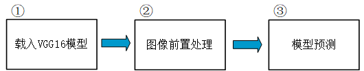
代码:
 1 # 完全采用 VGG 16 预先训练的模型
 2 # 载入套件
 3 import tensorflow as tf
 4 from tensorflow.keras.applications.vgg16 import VGG16
 5 from tensorflow.keras.preprocessing import image
 6 from tensorflow.keras.applications.vgg16 import preprocess_input
 7 from tensorflow.keras.applications.vgg16 import decode_predictions
 8 import numpy as np
 9
10 # 载入模型 模型路径 —— C-Users-guomi-.keras-models
11 model = VGG16(weights='imagenet')  # 16 = 13个卷积层 + 3个全连接层
12 print(model.summary())
13
14 # 绘制模型结构
15 tf.keras.utils.plot_model(model, to_file='vgg16.png')
16
17 # 模型预测
18 # 任选一张图片,例如大象侧面照
19 img_path = './data/images_test/elephant.jpg'
20 # 任选一张图片,例如大象正面照
21 # img_path = './data/images_test/elephant2.jpg'
22 img = image.load_img(img_path, target_size=(224, 224))  # 载入图档,并缩放宽高为 (224, 224)
23
24 x = image.img_to_array(img)    # 把PIL类型转换为numpy类型
25 x = np.expand_dims(x, axis=0)  # 加一维,变成 (1, 224, 224, 3)
26 x = preprocess_input(x)        # 对数据进行vgg16的预处理
27
28 # 预测
29 preds = model.predict(x)
30 # decode_predictions: 取得前 3 名的物件,每个物件属性包括 (类别代码, 名称, 机率)
31 print('Predicted:', decode_predictions(preds, top=3)[0])
预测图像和代码运行结果:
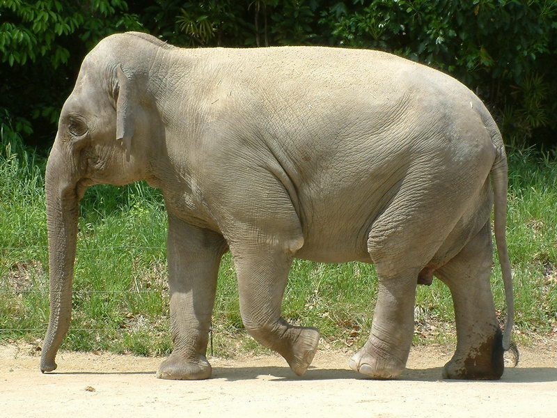
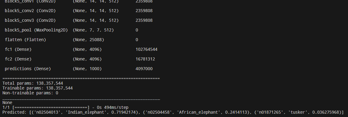
从结果可以看出,前三名的结果分别是印度象、非洲象、图斯克象。
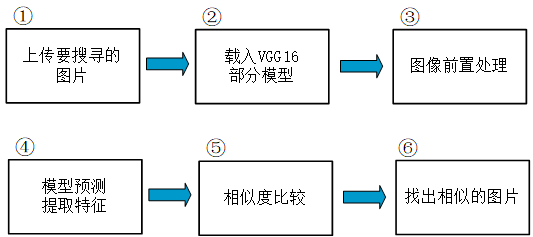
二、采用部分模型
预先训练模型的第二个用法,是采用部分模型,只提取特征,不做辨识。例如通过提取图片的特征来进行图片相似度的比较,从而推送出与该图片最相似的图片给用户。
设计思路:
代码:
1 # 图像相似度比较
2 # 载入套件
3 from tensorflow.keras.applications.vgg16 import VGG16
4 from tensorflow.keras.preprocessing import image
5 from tensorflow.keras.applications.vgg16 import preprocess_input
6 import numpy as np
7 from os import listdir
8 from os.path import isfile, join
9 # 使用 cosine_similarity 比较特征向量
10 from sklearn.metrics.pairwise import cosine_similarity
11
12 # 载入VGG 16 模型, 不含最上面的三层(辨识层)
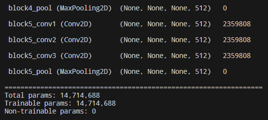
13 model = VGG16(weights='imagenet', include_top=False)
14 model.summary()
15
16 # 使用 cosine_similarity 比较特征向量
17 # 步骤 1. 取得 images_test 目录下所有 .jpg 档案名称
18 # 取得 images_test 目录下所有 .jpg 档案名称
19 img_path = 'data/images_test/'
20 image_files = np.array([f for f in listdir(img_path) if isfile(join(img_path, f)) and f[-3:] == 'jpg'])
21 print(image_files)
22
23 # 步骤 2. 取得 images_test 目录下所有 .jpg 档案的像素
24 # 合并所有图档的像素
25 X = np.array([])
26 for f in image_files:
27 image_file = join(img_path, f)
28 # 载入图档,并缩放宽高为 (224, 224)
29 img = image.load_img(image_file, target_size=(224, 224))
30 img2 = image.img_to_array(img) # 把PIL类型转换为numpy类型
31 img2 = np.expand_dims(img2, axis=0) # 加一维,变成 (1, 224, 224, 3)
32 # 保存所有图像的像素
33 if len(X.shape) == 1:
34 X = img2
35 else:
36 X = np.concatenate((X, img2), axis=0)
37
38 # 对图像进行预处理
39 X = preprocess_input(X)
40
41 # 步骤 3. 取得所有图档的特征向量
42 # 取得所有图档的特征向量
43 features = model.predict(X)
44 # 查看某个图档的特征向量
45 print(features[5])
46 print("特征图的大小 = ", features.shape, "原始图的大小 = ", X.shape)
47
48 # 步骤 4. 使用 cosine_similarity 函数比较特征向量
49 # 比较 Tiger2.jpg 与其他图档特征向量
50 no = -2
51 print(image_files[no])
52
53 # 转为二维向量,类似扁平层(Flatten) shape由原来的(16, 7, 7, 512)变成了(16, 25088)
54 features2 = features.reshape((features.shape[0], -1))
55 # 排除 Tiger2.jpg 的其他图档特征向量
56 other_features = np.concatenate((features2[:no], features2[no+1:]))
57 # 使用 cosine_similarity 计算 Cosine 函数
58 similar_list = cosine_similarity(features2[no:no+1], other_features, dense_output=False)
59
60 # 显示相似度,由大排到小 [::-1]表示倒序
61 print(np.sort(similar_list[0])[::-1])
62
63 # 依相似度,由大排到小,显示档名
64 image_files2 = np.delete(image_files, no)
65 print(image_files2[np.argsort(similar_list[0])[::-1]])
代码运行结果:
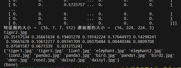
以上代码通过对不同的图像提取的特征做余弦函数相似度比较来找出与当前图像最相似的图像,如以上代码,和 tiger2.jpg 最相似的图像是 tiger1.jpg,其次是 tiger3.jpg,lion1.jpg,elephant.jpg,elephant2.jpg,以此类推。
三、采用部分模型+自定义层 —— 迁移学习
预先训练模型的第三种用法,是采用部分的模型,再加上自定义的输入层和辨识层,如此就能够不受限于模型原先辨识的对象,也就是所谓的转移学习(Transfer Learning),或者翻译为迁移学习。一般的迁移学习分为以下两阶段。
(1)建立预先训练的模型:如之前提到的 Keras Applications,还有在自然语言处理方面的 BERT,利用大量的训练数据和复杂模型结构,取得通用性的图像与自然语言特征向量。
(2)微调(Fine Tuning):利用预先训练模型的前半段,再加入自定义的神经层,进行特殊类别的辨识。
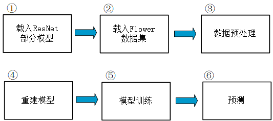
设计思路:
代码:
  1 # 自定的输入层及辨识层(Dense)
  2 import tensorflow as tf
  3 from tensorflow.keras.applications.resnet_v2 import ResNet152V2
  4 from tensorflow.keras.preprocessing import image
  5 from tensorflow.keras.applications.resnet_v2 import preprocess_input
  6 from tensorflow.keras.applications.resnet_v2 import decode_predictions
  7 from tensorflow.keras.layers import Dense, GlobalAveragePooling2D
  8 from tensorflow.keras.models import Model
  9 import numpy as np
 10 from tensorflow.keras import layers
 11 import matplotlib.pyplot as plt
 12
 13 # 步骤1:载入 Flower 资料
 14 # 资料集来源:https://www.tensorflow.org/tutorials/load_data/images
 15 # https://storage.googleapis.com/download.tensorflow.org/example_images/flower_photos.tgz
 16
 17 # 参数设定
 18 batch_size = 64
 19 img_height = 224
 20 img_width = 224
 21 data_dir = 'C://Users//guomi//.keras//datasets//flower_photos//'
 22
 23 # 载入 Flower 训练资料
 24 train_ds = tf.keras.preprocessing.image_dataset_from_directory(
 25   data_dir,
 26   validation_split=0.2,  # 0和1之间的可选浮点数,可保留一部分数据用于验证。
 27   subset="training",     # "training"或"validation"之一。仅在设置validation_split时使用。
 28   seed=123,              # 用于shuffle和转换的可选随机种子
 29   image_size=(img_height, img_width),  # 从磁盘读取数据后将其重新调整大小。默认(256,256)。由于管道处理的图像批次必须具有相同的大小,因此该参数必须提供。
 30   batch_size=batch_size)  # batch_size: 数据批次的大小。默认值:32
 31
 32 # 载入 Flower 验证资料
 33 val_ds = tf.keras.preprocessing.image_dataset_from_directory(
 34   data_dir,
 35   validation_split=0.2,
 36   subset="validation",
 37   seed=123,
 38   image_size=(img_height, img_width),
 39   batch_size=batch_size)
 40 # 共3670个文件,5种类别(class),其中20%=734作为验证集使用,80%=2936作为训练集使用.
 41 # 因返回的是没批的数据,所以 train_ds的长度=46 , val_ds的长度=12
 42
 43 # 步骤2:进行特征工程,将特征缩放成(0, 1)之间
 44 normalization_layer = tf.keras.layers.experimental.preprocessing.Rescaling(1./255)
 45 normalized_ds = train_ds.map(lambda x, y: (normalization_layer(x), y))
 46 normalized_val_ds = val_ds.map(lambda x, y: (normalization_layer(x), y))
 47
 48 # 步骤3:建立模型结构
 49 # 预先训练好的模型 -- ResNet152V2 - 共有 152 层卷积/池化层,再加上其他类型的神经层,总共有 566 层.
 50 # 设置 include_top=False,最后两层 GlobalAveragePooling 和 Dense 这两层会被移除。
 51 base_model = ResNet152V2(weights='imagenet', include_top=False)
 52 print(base_model.summary())
 53
 54 # 加上自定义的辨识层(Dense)
 55 x = base_model.output
 56 x = GlobalAveragePooling2D()(x)
 57 predictions = Dense(5, activation='softmax')(x)
 58
 59 # 指定自定义的输入层及辨识层(Dense)来重新搭建模型
 60 model = Model(inputs=base_model.input, outputs=predictions)
 61
 62 # 模型前段不需训练了
 63 for layer in base_model.layers:
 64     layer.trainable = False
 65
 66 # 设定优化器(optimizer)、损失函数(loss)、效能衡量指标(metrics)的类别
 67 model.compile(optimizer='rmsprop', loss='sparse_categorical_crossentropy', metrics=['accuracy'])
 68 model.summary()
 69
 70 # 步骤5:模型训练
 71 # 配置数据集以提高性能,设定快取(cache)、prefetch,以增进训练效率
 72 # 我们确保使用缓冲预获取,以便您可以从磁盘生成数据,而不会导致 I/O 阻塞。下面是加载数据时应当使用的两个重要方法。
 73 #   - 在第一个周期期间从磁盘加载图像后,Dataset.cache() 会将这些图像保留在内存中。这将确保在训练模型时数据集不会成为瓶颈。
 74 #     如果数据集太大无法装入内存,您也可以使用此方法创建高性能的磁盘缓存。
 75 #   - Dataset.prefetch() 会在训练时将数据预处理和模型执行重叠。特别是,该转换会使用后台线程和内部缓冲区在请求元素之前从输入数据集中预提取元素。
 76 #     要预提取的元素数量应等于(或可能大于)单个训练步骤使用的批次数。您可以手动调整这个值,或者将其设置为 tf.data.AUTOTUNE,这将提示 tf.data
 77 #     运行时在运行期间动态调整该值。
 78 AUTOTUNE = tf.data.AUTOTUNE
 79 normalized_ds = normalized_ds.cache().prefetch(buffer_size=AUTOTUNE)
 80 normalized_val_ds = normalized_val_ds.cache().prefetch(buffer_size=AUTOTUNE)
 81
 82 # 模型训练
 83 history = model.fit(normalized_ds, validation_data=normalized_val_ds, epochs=5)
 84
 85 # 步骤6:绘制训练时准确率/损失函数的变化
 86 print(history.history.keys())
 87 # 对训练过程的准确率绘图
 88 plt.rcParams['font.sans-serif'] = ['Microsoft JhengHei']
 89 plt.rcParams['axes.unicode_minus'] = False
 90
 91 plt.figure(figsize=(8, 6))
 92 plt.plot(history.history['accuracy'], 'r', label='训练准确率')
 93 plt.plot(history.history['val_accuracy'], 'g', label='验证准确率')
 94 plt.xlabel('Epoch')
 95 plt.ylabel('准确率')
 96 plt.legend()
 97
 98 plt.plot(history.history['loss'], label='训练损失')
 99 plt.plot(history.history['val_loss'], label='验证损失')
100 plt.xlabel('Epoch')
101 plt.ylabel('损失')
102 plt.legend()
103
104 # 步骤7:预测
105 # 显示辨识的类别
106 class_names = train_ds.class_names
107 print(class_names)
108
109 # 任选一张图片,例如玫瑰,进行预测
110 img_path = 'data/images_test/rose.png'
111 # 载入图档,并缩放宽高为 (224, 224)
112 img = image.load_img(img_path, target_size=(224, 224))
113
114 x = image.img_to_array(img)
115 x = np.expand_dims(x, axis=0)
116 x = preprocess_input(x)
117
118 # 预测
119 preds = model.predict(x)
120
121 # 显示预测结果
122 y_pred = [round(i * 100, 2) for i in preds[0]]
123 print(f'预测机率(%):{y_pred}')
124 print(f'预测类别:{class_names[np.argmax(preds)]}')
预测图像和代码运行结果:
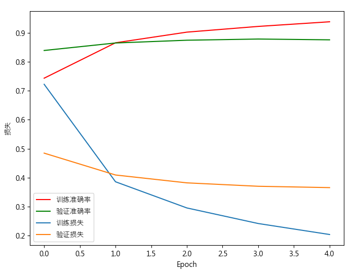
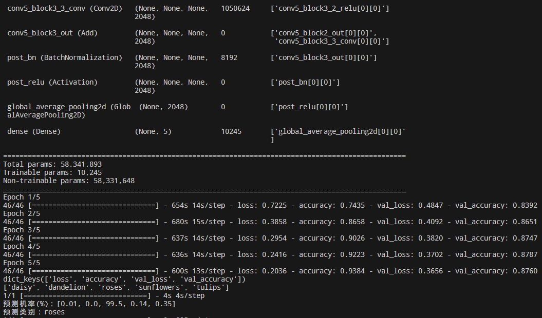
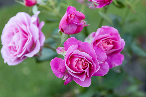
以上代码就实现了迁移学习,使用预训练模型的前半段,再加上自定义的辨识层。
本文所涉及到的数据集和模型可在如下地址进行下载:
链接:https://pan.baidu.com/s/1yRugo8YJJWu5lapS6qkOgw
提取码:4fi0
以上内容来自书籍《深度学习全书 公式+推导+代码+TensorFlow全程案例》—— 洪锦魁主编 清华大学出版社 ISBN 978-7-302-61030-4
- TensorFlow TensorFlow-Explanation 使用方法 Explanation pre-trainedtensorflow tensorflow-explanation使用方法 tensorflow-explanation explanation tensorflow模型 方法 explanation-aware explanation tokens json only explanation-aware environments explanation experience pre-trained pre-training 模型tensorflow2 tensorflow方法