horse or human
以下 python 代码将使用 OS 库来使用操作系统库,使您可以访问文件系统,并使用 zipfile 库来解压缩数据。
import os
import zipfile

local_zip = './tmp/horse-or-human.zip'
zip_ref = zipfile.ZipFile(local_zip, 'r')
zip_ref.extractall('./tmp/horse-or-human')
zip_ref.close()
.zip 的内容被提取到基本目录 ./tmp/horse-or- human(py中./表示上一级文件夹),该目录又包含 horses 和 humans 子目录。
简而言之:训练集是用来告诉神经网络模型“这就是马的样子”、“这就是人的样子”等的数据。
在这个示例中需要注意的一件事是:我们没有明确地将图像标记为马或人。如果你还记得之前的手写示例(Ex2),我们已经标记了“这是一个 1”、“这是一个 7”等。稍后你会看到使用了一个名为 ImageGenerator 的东西——它被编码为从子目录中读取图像,并自动根据该子目录的名称来标记它们。因此,例如,您将有一个“训练”目录,其中包含一个“马”目录和一个“人类”目录。 ImageGenerator 将为您适当地标记图像,从而减少编码步骤。
让我们定义每个目录:
# Directory with our training horse pictures
train_horse_dir = os.path.join('./tmp/horse-or-human/horses')

# Directory with our training human pictures
train_human_dir = os.path.join('./tmp/horse-or-human/humans')
现在,让我们看看马匹和人类训练目录中的文件名是什么样子的:
train_horse_names = os.listdir(train_horse_dir)
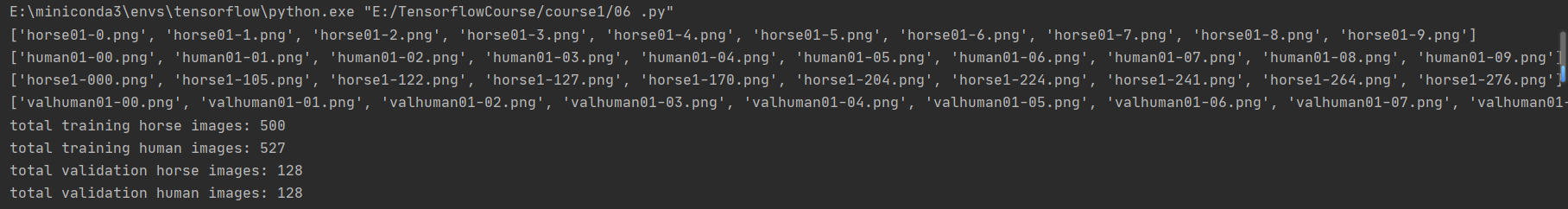
print(train_horse_names[:10])
train_human_names = os.listdir(train_human_dir)
print(train_human_names[:10])
让我们找出目录中马和人的图片总数:
print('total training horse images:', len(os.listdir(train_horse_dir)))
print('total training human images:', len(os.listdir(train_human_dir)))
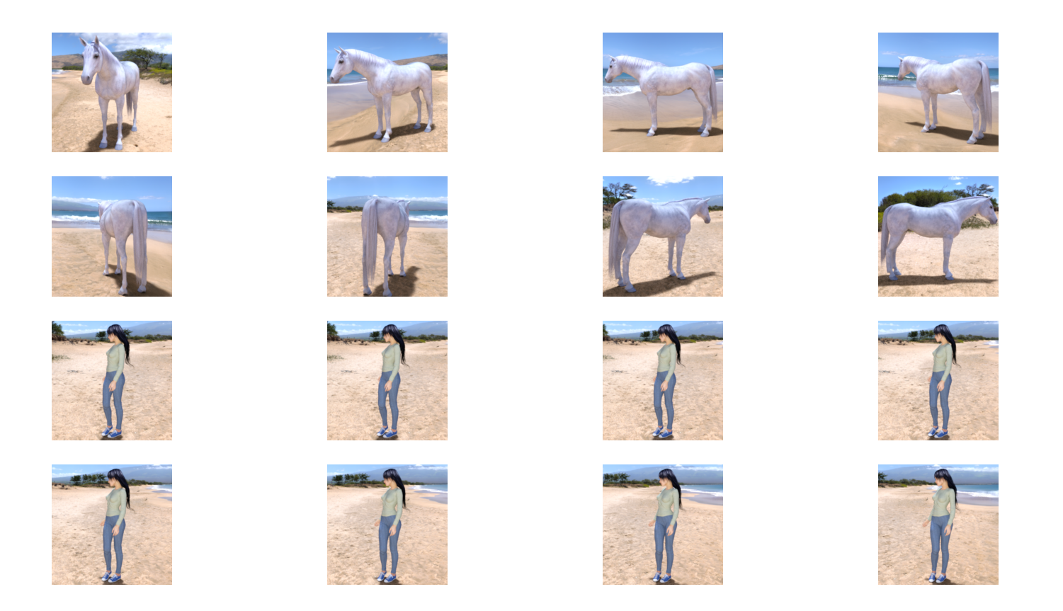
现在让我们看几张图片,以便更好地了解它们的外观。首先,配置 matplot 参数:
#%matplotlib inline

import matplotlib.pyplot as plt
import matplotlib.image as mpimg

# Parameters for our graph; we'll output images in a 4x4 configuration
nrows = 4
ncols = 4

# Index for iterating over images
pic_index = 0
现在,展示一批8匹马和8匹人的图片。您可以重新运行单元以每次查看新的批次:
# Set up matplotlib fig, and size it to fit 4x4 pics
fig = plt.gcf()
fig.set_size_inches(ncols * 4, nrows * 4)

pic_index += 8
next_horse_pix = [os.path.join(train_horse_dir, fname)
                for fname in train_horse_names[pic_index-8:pic_index]]
next_human_pix = [os.path.join(train_human_dir, fname)
                for fname in train_human_names[pic_index-8:pic_index]]

for i, img_path in enumerate(next_horse_pix+next_human_pix):
  # Set up subplot; subplot indices start at 1
  sp = plt.subplot(nrows, ncols, i + 1)
  sp.axis('Off') # Don't show axes (or gridlines)

  img = mpimg.imread(img_path)
  plt.imshow(img)

plt.show()
Building a Small Model from Scratch
但在继续之前,我们先来定义模型:
第一步是导入 tensorflow。
import tensorflow as tf
然后,我们像上一个例子一样添加卷积层,并将最终结果平铺到密集连接层中。
最后,我们添加密集连接层。
请注意,由于我们面对的是一个两类分类问题,即二元分类问题,因此我们将以一个 sigmoid 激活结束我们的网络,这样我们网络的输出将是一个介于 0 和 1 之间的单一标量,编码当前图像是类别 1(而不是类别 0)的概率。
model = tf.keras.models.Sequential([
    # Note the input shape is the desired size of the image 300x300 with 3 bytes color
    # This is the first convolution
    tf.keras.layers.Conv2D(16, (3,3), activation='relu', input_shape=(300, 300, 3)),
    tf.keras.layers.MaxPooling2D(2, 2),
    # The second convolution
    tf.keras.layers.Conv2D(32, (3,3), activation='relu'),
    tf.keras.layers.MaxPooling2D(2,2),
    # The third convolution
    tf.keras.layers.Conv2D(64, (3,3), activation='relu'),
    tf.keras.layers.MaxPooling2D(2,2),
    # The fourth convolution
    tf.keras.layers.Conv2D(64, (3,3), activation='relu'),
    tf.keras.layers.MaxPooling2D(2,2),
    # The fifth convolution
    tf.keras.layers.Conv2D(64, (3,3), activation='relu'),
    tf.keras.layers.MaxPooling2D(2,2),
    # Flatten the results to feed into a DNN
    tf.keras.layers.Flatten(),
    # 512 neuron hidden layer
    tf.keras.layers.Dense(512, activation='relu'),
    # Only 1 output neuron. It will contain a value from 0-1 where 0 for 1 class ('horses') and 1 for the other ('humans')
    tf.keras.layers.Dense(1, activation='sigmoid')
])
The model.summary() method call prints a summary of the NN
model.summary()
输出形状 "一栏显示了特征图的尺寸在每个连续层中的变化情况。卷积层由于填充作用,会将特征图的尺寸减小一些,而每个池化层则会将尺寸减半。
接下来,我们将配置模型训练的规格。我们将使用二元交叉熵损失(binary_crossentropy loss)来训练模型,因为这是一个二元分类问题,而我们的最终激活是一个 sigmoid。(我们将使用学习率为 0.001 的 rmsprop 优化器。在训练过程中,我们要监控分类的准确性。
注意:在这种情况下,使用 RMSprop 优化算法比使用随机梯度下降算法(SGD)更好,因为 RMSprop 可以自动调整学习率。(其他优化器,如 Adam 和 Adagrad,也能在训练过程中自动调整学习率,在此同样适用)。
from tensorflow.keras.optimizers import RMSprop

model.compile(loss='binary_crossentropy',
              optimizer=RMSprop(lr=0.001),
              metrics=['accuracy'])
Data Preprocessing
让我们建立数据生成器,读取源文件夹中的图片,将其转换为 float32 张量,然后将它们(连同标签)输入我们的网络。我们将使用一个生成器生成训练图片,另一个生成器生成验证图片。我们的生成器将生成一批大小为 300x300 的图像及其标签(二进制)。
正如你可能已经知道的,进入神经网络的数据通常应该以某种方式进行归一化处理,使其更适合网络处理。(在我们的案例中,我们将对图像进行预处理,将像素值归一化为 [0, 1] 范围内(最初所有值都在 [0, 255] 范围内)。
在 Keras 中,这可以通过 keras.preprocessing.image.ImageDataGenerator 类使用 rescale 参数来实现。该 ImageDataGenerator 类允许您通过 .flow(data, labels) 或 .flow_from_directory(directory) 来实例化增强图像批次(及其标签)的生成器。然后,这些生成器可用于接受数据生成器作为输入的 Keras 模型方法:fit、evaluate_generator 和 predict_generator。
from tensorflow.keras.preprocessing.image import ImageDataGenerator

# All images will be rescaled by 1./255
train_datagen = ImageDataGenerator(rescale=1/255)

# Flow training images in batches of 128 using train_datagen generator
train_generator = train_datagen.flow_from_directory(
        './tmp/horse-or-human/',  # This is the source directory for training images
        target_size=(300, 300),  # All images will be resized to 150x150
        batch_size=128,
        # Since we use binary_crossentropy loss, we need binary labels
        class_mode='binary')
Training
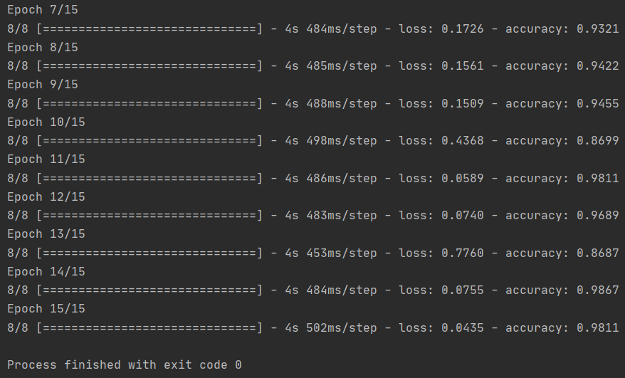
让我们训练 15 个 epoch——这可能需要几分钟才能运行。
请记下每个时期的值。
损失和准确度是训练进度的重要指标。它对训练数据的分类进行猜测,然后根据已知标签对其进行测量,计算结果。准确度是正确猜测的部分。
history = model.fit(
      train_generator,
      steps_per_epoch=8,
      epochs=15,
      verbose=1)
Running the Model
现在让我们看看如何使用该模型进行实际预测。这段代码将允许你从文件系统中选择 1 个或多个文件,然后上传这些文件,并通过模型运行这些文件,从而给出该对象是马还是人的指示。\