实验介绍:
利用数据集Fashion MNIST中的数据信息,进行机器学习,构建模型,训练模型。完成对该数据集中的数据分类(对运动鞋和衬衫等服装图像进行分类)。本实验主要使用 tf.keras,它是 TensorFlow 中用来构建和训练模型的高级 API。
导入 Fashion MNIST 数据:
头文件展示:
import tensorflow as tf
import numpy as np
import matplotlib.pyplot as plt
直接从 TensorFlow 中访问 Fashion MNIST。直接从 TensorFlow 中导入和加载 Fashion MNIST 数据,本数据集中包含了6000张训练数据和1000张测试数据:
fashion_mnist = tf.keras.datasets.fashion_mnist
(train_images, train_labels), (test_images, test_labels) = fashion_mnist.load_data()
为每一个标签(labels)命名:
#标签0-9分别对应的衣服
class_names = ['T-shirt/top', 'Trouser', 'Pullover', 'Dress', 'Coat',
               'Sandal', 'Shirt', 'Sneaker', 'Bag', 'Ankle boot']
标签命名前,标签命名后:

数据预处理一下,将这些值缩小至 0 到 1 之间,然后将其馈送到神经网络模型。为此,请将这些值除以 255。请务必以相同的方式对训练集和测试集进行预处理:
train_images = train_images / 255
test_images = test_images / 255
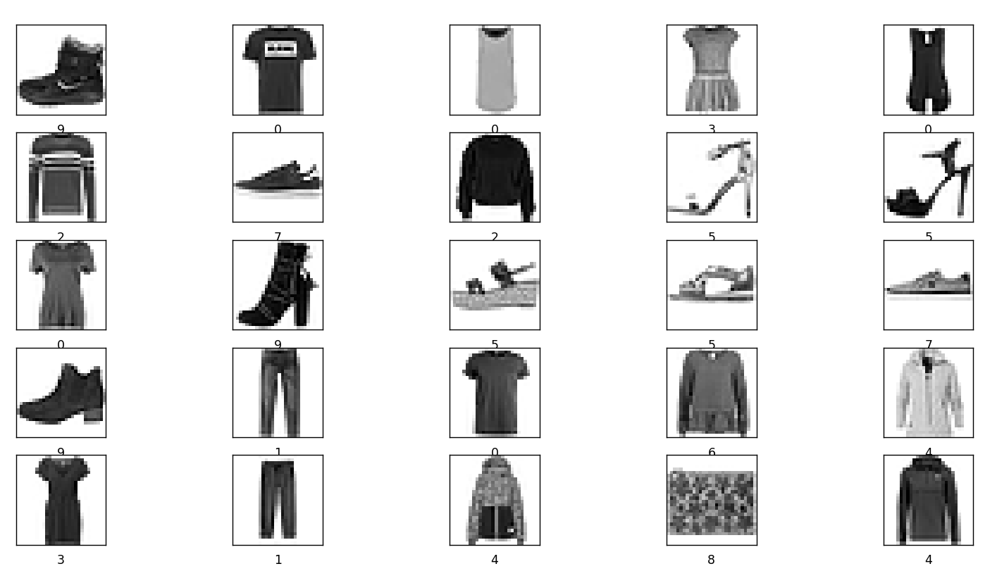
数据浏览,展示前25条数据:
plt.figure(figsize=(10,10))
for i in range(25):
    plt.subplot(5, 5, i + 1)
    plt.xticks([])
    plt.yticks([])
    # plt.cm.binary的作用是图片将以黑白色显示
    plt.imshow(train_images[i], cmap=plt.cm.binary)
    plt.xlabel(class_names[train_labels[i]])
plt.show()
构建模型:
设置层:
model = tf.keras.Sequential([
    tf.keras.layers.Flatten(input_shape=(28, 28)),
    tf.keras.layers.Dense(128, activation='relu'),
    tf.keras.layers.Dense(10)
])
编译模型:
model.compile(optimizer='adam',
              loss=tf.keras.losses.SparseCategoricalCrossentropy(from_logits=True),
              metrics=['accuracy'])
训练模型:
训练神经网络模型需要执行以下步骤:
- 将训练数据馈送给模型。在本例中,训练数据位于
train_images和train_labels数组中。 - 模型学习将图像和标签关联起来。
- 要求模型对测试集(在本例中为
test_images数组)进行预测。 - 验证预测是否与
test_labels数组中的标签相匹配。
训练模型:
model.fit(train_images, train_labels, epochs= 10)
模型测试:
test_loss, test_acc = model.evaluate(test_images, test_labels, verbose=2)
print("测试准确率为: ",test_acc)
模型预测:
先建立预测模型:
probability_model = tf.keras.Sequential([model,
                                         tf.keras.layers.Softmax()])
预测一下:
predictions = probability_model.predict(train_images)
看看预测的第一个数据怎么样:
predictions[0]
[2.1990630e-14 9.6575387e-11 8.7644484e-20 1.4134983e-15 3.9952511e-13
 2.2158854e-05 7.6434464e-14 8.5105496e-03 3.5996098e-14 9.9146724e-01]
可以发现,对于这个数据,是该模型预测出的该数据所属标签概率。
具体查看该数据最有可能的那个标签:
print(np.argmax(predictions[0]))
9
实验结束。