飞机基础知识一 1.3二维平面飞机运动学模型

飞机基础知识一 1.3二维平面飞机运动学模型
- 运动学方程
- 程序实现
  - 完整代码
  - 效果

运动学方程

在二维平面上

将飞机视为一个质点

\[\begin{aligned} & \frac{d x}{d t}=v \cos \psi \\ & \frac{d y}{d t}=v \sin \psi \\ & \frac{d v}{d t}= a \\ & \frac{d \psi}{d t}= \omega \\ \end{aligned} \]

状态量为位置 x ，y , 速率 v 速度与x轴的夹角 \(\theta\)

控制量为加速度大小 \(a\) 和角加速度大小 \(\omega\)

程序实现

给定初始状态

二维空间坐标值、飞行速率、与x轴夹角

\[x,y,v,\theta \]

state = [x,y,v,theta]

输入：控制量加速度和角加速度

\[a, \omega \]

control = [a , moega]

代码返回：下一时间（一个仿真步长）的状态量

完整代码

# -*- coding: utf-8 -*-

"""
@author     : zuti
@software   : PyCharm
@file       : 2_run_func.py
@time       : 2023/3/25 14:58
@desc       ：

"""

import matplotlib.pyplot as plt
import numpy as np



plt.rcParams['font.sans-serif'] = ['SimHei']
plt.rcParams['axes.unicode_minus'] = False
plt.rcParams.update({'font.size': 12})

# 初始姿态
init_velocity, init_theta  = 100., np.pi/2
init_x, init_y = 0., 0.  # 初始位置

# todo 两个控制量
a = 5.  #单位  m/s2
omega = 1   #单位 rad/s2

state = [init_x, init_y,  init_velocity, init_theta]
control = [a,omega]

time = 1  # 秒 总时间
n = 10  # 仿真步数
t = np.linspace(0, time, n)  # 仿真步长

def update_position(state, control, time=1, n=100):
    """

    :param state:  初始状态
    :param control: 控制量
    :param time:   仿真时长
    :param n: 仿真步数
    :return:
    """
    t = np.linspace(0, time, n)  # 仿真步长
    dt = t[1] - t[0]
    state_list = np.zeros((n, 4))  # 轨迹长度
    state_list[0] = state  # 轨迹列表第一个元素为初始状态
    x,y,velocity, theta = state_list[0]

    for k in range(1, n):

        a  =   control[0]
        omega = control[1]

        velocity = velocity +   a * dt
        theta= theta+ omega * dt


        dx = velocity * np.cos(theta) * dt
        dy = velocity * np.sin(theta) * dt


        x = x + dx
        state_list[k, 0] = x
        y = y + dy
        state_list[k, 1] = y


        state_list[k, 2] = velocity
        state_list[k, 3] =  theta

    return state_list

#测试运动学方程
state_list = update_position(state,control)
print(f'轨迹 {state_list}')
#绘制图像
fig = plt.figure()
ax1 = fig.add_subplot(221)
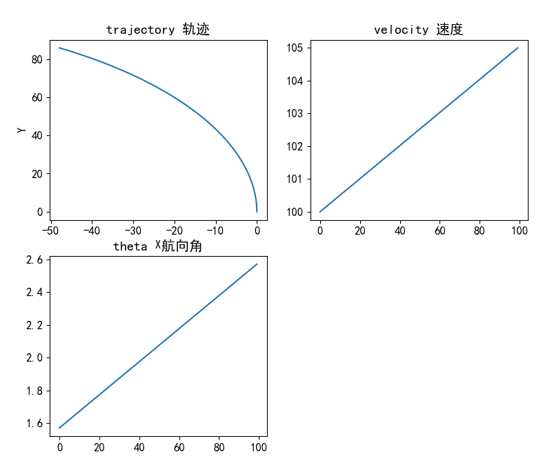
ax1.plot(state_list[:, 0], state_list[:, 1])
ax1.set_title('trajectory 轨迹')
ax1.set_xlabel('X')
ax1.set_ylabel('Y')


ax2 = fig.add_subplot(222)
ax2.plot(state_list[:,2])
ax2.set_title('velocity 速度')


ax3 = fig.add_subplot(223)
ax3.plot(state_list[:,3])
ax3.set_title('theta  航向角')

#plt.savefig('test.jpg')
plt.show()