机器学习 房价预测
选题背景
1) CRIM:每个城镇的人均犯罪率。这个属性表示每个城镇中每个人的犯罪率。它提供了有关该地区犯罪活动水平的信息。
2) CHAS:二元变量,决定每个城镇的土地是否位于查尔斯河的边界上。如果通道与河流接触,它的值为1,否则为0。它表明这个城镇离河很近。
3) ZN:分配给大型地块的住宅用地比例。
4) INDUS:每个城镇非零售商业用地的百分比。
5) NOX:空气中一氧化氮的浓度水平,单位为千万分之一。
6) RM:在每个城镇的住宅中发现的平均房间数
7)年龄:1940年以前建造的自住单位的百分比。
8) DIS:到波士顿五个就业中心的加权距离。
9)RAD:表示从每个城镇到径向高速公路的方便程度的量化指数
10)税收:按每$10,000的全部财产价值计算的房产税率。
关于税务的更多信息:https://www.rocketmortgage.com/learn/property-tax
PTRATIO:按城镇划分的师生比例。
12) B: 1000(Bk - 0.63)^2,其中Bk是按城镇划分的黑人比例。
13) LSTAT:人口地位降低%。
14)MEDV:自住房屋价值中位数,以1000美元计*
from pathlib import Pathimport re
import numpy as np from scipy import statsimport pandas as pd import matplotlib.pyplot as pltimport seaborn as snsimport tqdm.auto as tqdm
/opt/conda/lib/python3.10/site-packages/scipy/__init__.py:146: UserWarning: A NumPy version >=1.16.5 and <1.23.0 is required for this version of SciPy (detected version 1.23.5
warnings.warn(f"A NumPy version >={np_minversion} and <{np_maxversion}"
file_names = list(Path('/kaggle/input').rglob('*.csv'))file = file_names[0]
df = pd.read_csv(file)
探索性数据分析(EDA)/描述性方法
#最初声明目标特性,因为它将被进一步使用。
target = 'MEDV'
#有多个特征从中位数有很高的分布,表明一个很高的右/左偏度。
#这将被记录为稍后将应用的不倾斜策略。
df.describe()
# CHAS Feature是二进制的,但是在原始数据集中没有这样表示
df.dtypes

#有多个特征缺少数据,幸运的是,
#所有的特征都是数值的,可以使用中值填充方法。
df.info ()

df.nunique()

def plot_hist(df):
    # Selecting numerical features, this is not required as all features
    # are numerical
    cols = (
        df
        .select_dtypes(include=[int, float])
        .columns
    )

    ncols = 2
    # Determining how many rows will be required based on the number of features
    # that are available; this process is agile and won't require modifications
    # if new features will be added
    nrows = np.ceil(len(cols) / ncols).astype(int)
    # The more features there are available the larger the figure will become
    vertical_figsize = 2 * nrows

    axs = plt.subplots(nrows, ncols, figsize=[10, vertical_figsize])[1].flatten()

    for col, ax in zip(cols, axs):
        df[col].plot.hist(title=col, ax=ax)
    plt.tight_layout()
    plt.show()
plot_hist(df)

如前所述,预测有多个特征是高度不倾斜的;为了提高模型性能,需要去除异常值,使数据更具可解释性。
处理数据
#如前所述,NaN值将被中位数取代
df = df.fillna(df.median(axis=0))
df['CHAS'] = df['CHAS'].astype(bool)
功能建设
cri_zn:这个交互术语描述了人均犯罪率和超过25000平方英尺的住宅用地比例之间的关系。它探讨了大型住宅地块的可用性如何影响犯罪率。
INDUS_CHAS:这个交互项考察了每个城镇的非零售商业面积比例与查尔斯河的存在之间的关系。它调查了河流的存在如何影响该地区非零售商业用地的比例。
NOX_DIS:这个交互项探讨了空气中一氧化氮浓度与波士顿五个主要就业中心的加权距离之间的关系。它调查了空气污染水平如何根据离就业中心的远近而变化。
RM_AGE:这个相互作用项考察了每个住宅的平均房间数与1940年以前建造的自住单位比例之间的关系。它探讨了住宅中房间的数量如何受到自住单位年龄的影响。
RAD_TAX:这个交互项研究径向高速公路可达性指数与每10,000美元的全额房产税率之间的关系。它探讨了径向高速公路的可达性如何影响该地区的房产税率。
PTRATIO_B:这个交互项探讨了城镇师生比例与涉及黑人居民比例的项之间的关系。它调查了城镇的人口构成,特别是黑人居民的比例,如何在塑造教育环境中与师生比例相互作用。
df['CRIM_ZN'] = df['CRIM'] * df['ZN']df['INDUS_CHAS'] = df['INDUS'] * df['CHAS']df['NOX_DIS'] = df['NOX'] * df['DIS']df['RM_AGE'] = df['RM'] * df['AGE']df['RAD_TAX'] = df['RAD'] * df['TAX']df['PTRATIO_B'] = df['PTRATIO'] * df['B']
Unskewing数据
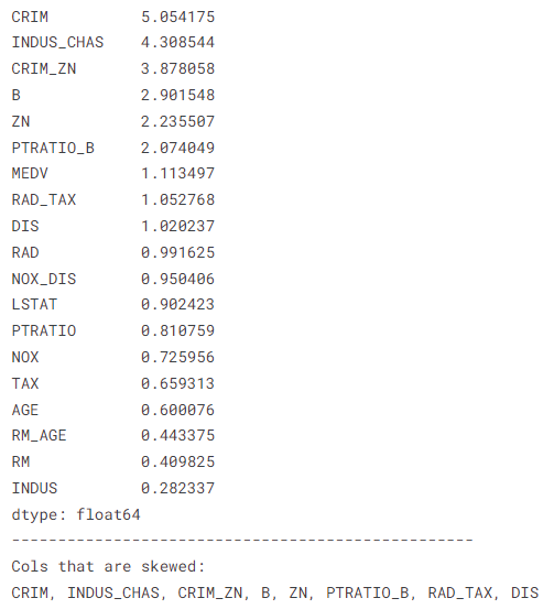
skew_res = df.select_dtypes([int, float]).skew().abs().sort_values(ascending=False)skew_cols = skew_res.loc[lambda x: (x>=1) & (x.index!=target)].index
print(skew_res)print('-'*50)print('Cols that are skewed:')print(', '.join(skew_cols))
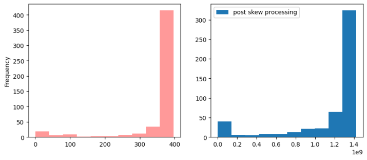
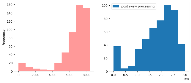
def best_transformation(data) -> tuple:
    functions = [np.log1p, np.sqrt, stats.yeojohnson]
    results = []

    for func in functions:
        transformed_data = func(data)
        if type(transformed_data) == tuple:
            vals, _ = transformed_data
            results.append(vals)
        else:
            results.append(transformed_data)

    abs_skew_results = [np.abs(stats.skew(val)) for val in results]
    lowest_skew_index = abs_skew_results.index(min(abs_skew_results))
    return functions[lowest_skew_index], results[lowest_skew_index]
def unskew(col):
    global best_transformation
    print('-'*100)
    col_skew = stats.skew(col)
    col_name = col.name
    print('{} skew is: {}'.format(col_name, col_skew))
    fig, (ax1, ax2) = plt.subplots(1, 2, figsize=[10, 4])
    col.plot.hist(color='red', alpha=.4, label='pre-skew', ax=ax1)

    if np.abs(col_skew) >= 1.:
        result_skew, data = best_transformation(col)
        new_col_skew = stats.skew(data)
        print(f'Best function {result_skew} and the skew results: {new_col_skew}')
        ax2.hist(data, label='post skew processing')
        plt.legend()
        plt.show()

        if np.abs(new_col_skew) >= 1.:
            print(f'Transformation was not successful for {col_name}, returning original data')
            return col

        return data

    plt.show()
    df[skew_cols] = df[skew_cols].apply(unskew, axis=0);
----------------------------------------------------------------------------------------------------
CRIM偏差为:5.039268385290411
最佳函数<function yeojohnson at 0x7db1c918ae60>和偏差结果:0.591919839543328

INDUS_CHAS偏差为4.2958364268220945
最佳函数<function yeojohnson at 0x7db1c918ae60>和歪斜结果:3.4083448897268838

对INDUS_CHAS的转换不成功,返回原始数据
----------------------------------------------------------------------------------------------------
CRIM_ZN偏差为:3.8666200276645553
最佳函数<function yeojohnson at 0x7db1c918ae60>和歪斜结果:1.117940048429315

转换对CRIM_ZN不成功,返回原始数据
----------------------------------------------------------------------------------------------------
B斜:-2.8929901521077115
最佳函数<函数yeojohnson在0x7db1c918ae60>和歪斜结果:-1.912938918160781
B转换不成功,返回原始数据
----------------------------------------------------------------------------------------------------
ZN偏度为:2.2289141017520993
最佳函数<function yeojohnson at 0x7db1c918ae60>和歪斜结果:1.0775267223714033

ZN转换不成功,返回原始数据
----------------------------------------------------------------------------------------------------
PTRATIO_B偏差为:-2.067932021002207
最佳函数<function yeojohnson at 0x7db1c918ae60>和歪斜结果:-0.8972822949834165
----------------------------------------------------------------------------------------------------
RAD_TAX偏差是:1.0496626140364416
最佳函数<function yeojohnson at 0x7db1c918ae60>和偏差结果:0.06768725522055934

----------------------------------------------------------------------------------------------------
DIS偏差为:1.0172283893817673
最佳函数<function yeojohnson at 0x7db1c918ae60>和歪斜结果:0.06811069535507755

属性链路选择
选择与目标相关度最高的数据
corr_ranking = (
    df
    .drop(target, axis=1)
    .corrwith(df[target])
    .abs()
    .sort_values(ascending=False))
_, ax = plt.subplots(figsize=[10, 10])sns.heatmap(df.corr(), annot=True, cmap="rocket", cbar=False, ax=ax);

相关系数在0.9和1.0之间表示变量可以被认为是高度相关的。相关系数在0.7 ~ 0.9之间表示变量可以认为是高度相关的。相关系数在0.5到0.7之间表示变量可以被认为是适度相关的。相关系数在0.3 ~ 0.5之间表示变量相关性较低。相关系数小于0.3的相关系数几乎没有(线性)相关。我们可以很容易地看到,0.9 < |r| < 1.0对应0.81 < r2 < 1.00;0.7 < |r| < 0.9对应0.49 < r2 < 0.81;0.5 < |r| < 0.7对应0.25 < r2 < 0.49;0.3 < |r| < 0.5对应0.09 < r2 < 0.25;0.0 < |r| < 0.3对应0.0 < r2 < 0.09。
#取0.3以上的所有值
threshold = .3chosen_cols = corr_ranking[corr_ranking>=threshold]print(chosen_cols)chosen_cols = chosen_cols.index.to_list()

数据准备/机器学习
训练测试数据分割
X = df[chosen_cols]y = df[target]
X.shape, y.shape

from sklearn.model_selection import train_test_split
X_train, X_test, y_train, y_test = train_test_split(X, y)
扩展

#由于CHAS没有通过相关过滤,所以没有必要删除它
from sklearn.preprocessing import StandardScaler
scaler = StandardScaler()
cols = X_train.select_dtypes([float, int]).columns.to_list()
X_train[cols] = scaler.fit_transform(X_train)X_test[cols] = scaler.transform(X_test)
模型构建(回归)/非描述性方法
from sklearn.linear_model import LinearRegressionfrom sklearn.ensemble import RandomForestRegressorfrom xgboost import XGBRegressor
from sklearn.experimental import enable_halving_search_cvfrom sklearn.model_selection import HalvingGridSearchCV
n_features = X_train.shape[1]
linear_reg_params = {
    'fit_intercept': [True, False],}
random_forest_params = {
    'n_estimators': np.sort(np.random.default_rng().choice(500, size=10, replace=False)),
    'max_features': np.sort(np.random.default_rng().choice(n_features, size=5, replace=False)),
    'max_depth': [1, 5, 10],}
xgb_params = {
    'objective': ['reg:squarederror'],
    'max_depth': [2, 5,],
    'min_child_weight': np.arange(1, 5, 2),
    'n_estimators': np.sort(np.random.default_rng().choice(500, size=3, replace=False)),
    'learning_rate': [1e-1, 1e-2,],
    'gamma': np.sort(np.random.default_rng().choice(20, size=3, replace=False)),
    'reg_lambda': [0, 1.0, 10.0],
    'scale_pos_weight': [1, 3, 5],
    'n_jobs': [-1],}
best_mode_params = {
    LinearRegression(): {'fit_intercept': True},
    RandomForestRegressor(): {'max_depth': 10, 'max_features': 9, 'n_estimators': 378},
    XGBRegressor(): {'gamma': 18, 'learning_rate': 0.1, 'max_depth': 2, 'min_child_weight': 3, 'n_estimators': 461, 'n_jobs': -1, 'objective': 'reg:squarederror', 'reg_lambda': 0, 'scale_pos_weight': 1},}
from sklearn.metrics import mean_squared_error, r2_scoreb_models = []model_results = []
for model in best_mode_params.keys():
    params = best_mode_params[model]
    model.set_params(**params)
    model.fit(X_train, y_train)
    b_models.append(model)

    y_pred = model.predict(X_test)
    mse = mean_squared_error(y_test, y_pred)
    rmse = np.sqrt(mse)
    r2 = r2_score(y_test, y_pred)

    model_name = re.search(r'\w+', str(model))[0]
    results = pd.Series({'MSE': mse, 'RMSE': rmse, 'R2': r2}, name=model_name)
model_results.append(results)
评估
pd.concat(model_results, axis=1)

从上面可以看出,XGBoost优于RandomForest。
feature_imp = []for model in b_models:
    try:
        model_name = re.search(r'\w+', str(model))[0]
        feature_imp.append(
            pd.Series(
                {
                    col: importance
                    for col, importance in zip(cols, model.feature_importances_)
                },
                name = model_name
            )
        )
    except AttributeError:
        pass
    pd.concat(feature_imp, axis=1).sort_values(by='XGBRegressor', ascending=False)

RM在特征重要性方面出人意料地超过了LSTAT,尽管LSTAT与目标的相关性更强。目前,通过将实际数据与模型的预测绘制成图形,提供模型性能的直观表示是可行的。
xgb_model = b_models[2]col = 'LSTAT'y_pred = xgb_model.predict(X_test.sort_values(by=col))
(
    pd.concat([X_test[col], y_test], axis=1)
    .sort_values(by=col)
    .plot(x=col, y='MEDV', color='red', alpha=.4, label='Actual Data'),)
plt.scatter(X_test[col].sort_values(), y_pred, label='Prediction Data')plt.legend()plt.show()

最终结果
手册中的数据经过了全面的分析和处理程序,从而开发出可靠的模型。评价结果证明了这些模型在生成准确预测方面的有效性。然而,仍有进一步改进的潜力。为了更有效地解决这个问题,在进行超参数调优之前,利用一个比较不同模型的工具将是有利的。该方法可以选择最优模型,提高预测模型的整体性能
已经实现了一个描述性方法
一个Non-Descriptive
机器学习已经被应用
已采取适当的保安措施。
显示了用于查看数据和遍历解析集的接口。
所有代码
from pathlib import Pathimport re
import numpy as np from scipy import statsimport pandas as pd import matplotlib.pyplot as pltimport seaborn as snsimport tqdm.auto as tqdm
file_names = list(Path('/kaggle/input').rglob('*.csv'))file = file_names[0]
df = pd.read_csv(file)
#最初声明目标特性,因为它将被进一步使用。
target = 'MEDV'
#有多个特征从中位数有很高的分布,表明一个很高的右/左偏度。
#这将被记录为稍后将应用的不倾斜策略。
df.describe ()
# CHAS Feature是二进制的,但是在原始数据集中没有这样表示
df.dtypes
#有多个特征缺少数据,幸运的是,
#所有的特征都是数值的,可以使用中值填充方法。
df.info ()
df.nunique()
def plot_hist(df):
#选择数字特征,这不是所有特征所必需的
#是数字
 cols = (
        df
        .select_dtypes(include=[int, float])
        .columns
    )

    ncols = 2
#根据特征的数量决定需要多少行
#可用的;这个过程是敏捷的,不需要修改
#如果将添加新功能
 nrows = np.ceil(len(cols) / ncols).astype(int)
#可用的特性越多,数字就越大
 vertical_figsize = 2 * nrows

    axs = plt.subplots(nrows, ncols, figsize=[10, vertical_figsize])[1].flatten()

    for col, ax in zip(cols, axs):
        df[col].plot.hist(title=col, ax=ax)
    plt.tight_layout()
    plt.show()
plot_hist(df)
#如前所述,NaN值将被中位数取代
df = df.fillna(df.median(axis=0))
df['CHAS'] = df['CHAS'].astype(bool)
df['CRIM_ZN'] = df['CRIM'] * df['ZN']df['INDUS_CHAS'] = df['INDUS'] * df['CHAS']df['NOX_DIS'] = df['NOX'] * df['DIS']df['RM_AGE'] = df['RM'] * df['AGE']df['RAD_TAX'] = df['RAD'] * df['TAX']df['PTRATIO_B'] = df['PTRATIO'] * df['B']
skew_res = df.select_dtypes([int, float]).skew().abs().sort_values(ascending=False)skew_cols = skew_res.loc[lambda x: (x>=1) & (x.index!=target)].index
print(skew_res)print('-'*50)print('Cols that are skewed:')print(', '.join(skew_cols))
def best_transformation(data) -> tuple:
    functions = [np.log1p, np.sqrt, stats.yeojohnson]
    results = []

    for func in functions:
        transformed_data = func(data)
        if type(transformed_data) == tuple:
            vals, _ = transformed_data
            results.append(vals)
        else:
            results.append(transformed_data)

    abs_skew_results = [np.abs(stats.skew(val)) for val in results]
    lowest_skew_index = abs_skew_results.index(min(abs_skew_results))
    return functions[lowest_skew_index], results[lowest_skew_index]
def unskew(col):
    global best_transformation
    print('-'*100)
    col_skew = stats.skew(col)
    col_name = col.name
    print('{} skew is: {}'.format(col_name, col_skew))
    fig, (ax1, ax2) = plt.subplots(1, 2, figsize=[10, 4])
    col.plot.hist(color='red', alpha=.4, label='pre-skew', ax=ax1)

    if np.abs(col_skew) >= 1.:
        result_skew, data = best_transformation(col)
        new_col_skew = stats.skew(data)
        print(f'Best function {result_skew} and the skew results: {new_col_skew}')
        ax2.hist(data, label='post skew processing')
        plt.legend()
        plt.show()

        if np.abs(new_col_skew) >= 1.:
            print(f'Transformation was not successful for {col_name}, returning original data')
            return col

        return data

    plt.show()
    df[skew_cols] = df[skew_cols].apply(unskew, axis=0);
corr_ranking = (
    df
    .drop(target, axis=1)
    .corrwith(df[target])
    .abs()
    .sort_values(ascending=False))
_, ax = plt.subplots(figsize=[10, 10])sns.heatmap(df.corr(), annot=True, cmap="rocket", cbar=False, ax=ax);
#取0.3以上的所有值
threshold = .3chosen_cols = corr_ranking[corr_ranking>=threshold]print(chosen_cols)
chosen_cols = chosen_cols.index.to_list()
X = df[chosen_cols]y = df[target]
X.shape, y.shape
from sklearn.model_selection import train_test_split
X_train, X_test, y_train, y_test = train_test_split(X, y)
X_train.dtypes
#由于CHAS没有通过相关过滤,所以没有必要删除它
from sklearn.preprocessing import StandardScaler
scaler = StandardScaler()
cols = X_train.select_dtypes([float, int]).columns.to_list()
X_train[cols] = scaler.fit_transform(X_train)X_test[cols] = scaler.transform(X_test)
from sklearn.linear_model import LinearRegressionfrom sklearn.ensemble import RandomForestRegressorfrom xgboost import XGBRegressor
from sklearn.experimental import enable_halving_search_cvfrom sklearn.model_selection import HalvingGridSearchCV
n_features = X_train.shape[1]
linear_reg_params = {
    'fit_intercept': [True, False],}
random_forest_params = {
    'n_estimators': np.sort(np.random.default_rng().choice(500, size=10, replace=False)),
    'max_features': np.sort(np.random.default_rng().choice(n_features, size=5, replace=False)),
    'max_depth': [1, 5, 10],
xgb_params = {
    'objective': ['reg:squarederror'],
    'max_depth': [2, 5,],
    'min_child_weight': np.arange(1, 5, 2),
    'n_estimators': np.sort(np.random.default_rng().choice(500, size=3, replace=False)),
    'learning_rate': [1e-1, 1e-2,],
    'gamma': np.sort(np.random.default_rng().choice(20, size=3, replace=False)),
    'reg_lambda': [0, 1.0, 10.0],
    'scale_pos_weight': [1, 3, 5],
    'n_jobs': [-1],}
best_mode_params = {
    LinearRegression(): {'fit_intercept': True},
    RandomForestRegressor(): {'max_depth': 10, 'max_features': 9, 'n_estimators': 378},
    XGBRegressor(): {'gamma': 18, 'learning_rate': 0.1, 'max_depth': 2, 'min_child_weight': 3, 'n_estimators': 461, 'n_jobs': -1, 'objective': 'reg:squarederror', 'reg_lambda': 0, 'scale_pos_weight': 1},}
from sklearn.metrics import mean_squared_error, r2_scoreb_models = []model_results = []
for model in best_mode_params.keys():
    params = best_mode_params[model]
    model.set_params(**params)
    model.fit(X_train, y_train)
    b_models.append(model)

    y_pred = model.predict(X_test)
    mse = mean_squared_error(y_test, y_pred)
    rmse = np.sqrt(mse)
    r2 = r2_score(y_test, y_pred)

    model_name = re.search(r'\w+', str(model))[0]
    results = pd.Series({'MSE': mse, 'RMSE': rmse, 'R2': r2}, name=model_name)
    model_results.append(results)
pd.concat(model_results, axis=1)
feature_imp = []for model in b_models:
    try:
        model_name = re.search(r'\w+', str(model))[0]
        feature_imp.append(
            pd.Series(
                {
                    col: importance
                    for col, importance in zip(cols, model.feature_importances_)
                },
                name = model_name
            )
        )
    except AttributeError:
        pass
pd.concat(feature_imp, axis=1).sort_values(by='XGBRegressor', ascending=False)

xgb_model = b_models[2]col = 'LSTAT'y_pred = xgb_model.predict(X_test.sort_values(by=col))
(
    pd.concat([X_test[col], y_test], axis=1)
    .sort_values(by=col)
    .plot(x=col, y='MEDV', color='red', alpha=.4, label='Actual Data'),)
plt.scatter(X_test[col].sort_values(), y_pred, label='Prediction Data')plt.legend()plt.show()