2.2.1 函数调用:pyplot、pylab
- pylot: 创建画板、示例图
- pylab: 结合pyplot和numpy函数的调用,功能比较复杂,不建议使用
2.2.2 创建画板(操作对象)
- plt.figure,设置图形大小,返回figure画板对象
- plt.subplots,设置行数、列表,创建相应数量的axes对象
2.2.3 生成图表
2.2.4 配置图例
- title,设置图表标题
- axis/xlim/ylim:设置坐标轴范围
- grid: 添加图标网格线
- legend: 添加label图例参数并显示
- xlabel/ylabel: 设置x.y轴标题
- xticks/yticks: 定义坐标轴刻度显示
- text/arrow/annotation: 分别在图例指定位置添加文字、箭头和标记
In [2]:
pip install matplotlib
Requirement already satisfied: matplotlib in c:\users\dengzl\.conda\envs\data_analysis\lib\site-packages (3.8.0)
Requirement already satisfied: contourpy>=1.0.1 in c:\users\dengzl\.conda\envs\data_analysis\lib\site-packages (from matplotlib) (1.1.1)
Requirement already satisfied: cycler>=0.10 in c:\users\dengzl\.conda\envs\data_analysis\lib\site-packages (from matplotlib) (0.12.1)
Requirement already satisfied: fonttools>=4.22.0 in c:\users\dengzl\.conda\envs\data_analysis\lib\site-packages (from matplotlib) (4.43.1)
Requirement already satisfied: kiwisolver>=1.0.1 in c:\users\dengzl\.conda\envs\data_analysis\lib\site-packages (from matplotlib) (1.4.5)
Requirement already satisfied: numpy<2,>=1.21 in c:\users\dengzl\.conda\envs\data_analysis\lib\site-packages (from matplotlib) (1.26.0)
Requirement already satisfied: packaging>=20.0 in c:\users\dengzl\.conda\envs\data_analysis\lib\site-packages (from matplotlib) (23.1)
Requirement already satisfied: pillow>=6.2.0 in c:\users\dengzl\.conda\envs\data_analysis\lib\site-packages (from matplotlib) (10.0.1)
Requirement already satisfied: pyparsing>=2.3.1 in c:\users\dengzl\.conda\envs\data_analysis\lib\site-packages (from matplotlib) (3.1.1)
Requirement already satisfied: python-dateutil>=2.7 in c:\users\dengzl\.conda\envs\data_analysis\lib\site-packages (from matplotlib) (2.8.2)
Requirement already satisfied: importlib-resources>=3.2.0 in c:\users\dengzl\.conda\envs\data_analysis\lib\site-packages (from matplotlib) (6.1.0)
Requirement already satisfied: zipp>=3.1.0 in c:\users\dengzl\.conda\envs\data_analysis\lib\site-packages (from importlib-resources>=3.2.0->matplotlib) (3.11.0)
Requirement already satisfied: six>=1.5 in c:\users\dengzl\.conda\envs\data_analysis\lib\site-packages (from python-dateutil>=2.7->matplotlib) (1.16.0)
Note: you may need to restart the kernel to use updated packages.
In [2]:
import matplotlib.pyplot as plt
# 创建figure、subplots
plt.subplots
Out[2]:
<function matplotlib.pyplot.subplots(nrows: 'int' = 1, ncols: 'int' = 1, *, sharex: "bool | Literal['none', 'all', 'row', 'col']" = False, sharey: "bool | Literal['none', 'all', 'row', 'col']" = False, squeeze: 'bool' = True, width_ratios: 'Sequence[float] | None' = None, height_ratios: 'Sequence[float] | None' = None, subplot_kw: 'dict[str, Any] | None' = None, gridspec_kw: 'dict[str, Any] | None' = None, **fig_kw) -> 'tuple[Figure, Any]'>
In [3]:
plt.subplots(2,1,True)
---------------------------------------------------------------------------
TypeError                                 Traceback (most recent call last)
Cell In[3], line 1
----> 1 plt.subplots(2,1,True)

TypeError: subplots() takes from 0 to 2 positional arguments but 3 were given
In [4]:
plt.subplots(2,1)
Out[4]:
(<Figure size 640x480 with 2 Axes>, array([<Axes: >, <Axes: >], dtype=object))
In [5]:
plt.subplots(2,1,sharex=true)
---------------------------------------------------------------------------
NameError                                 Traceback (most recent call last)
Cell In[5], line 1
----> 1 plt.subplots(2,1,sharex=true)

NameError: name 'true' is not defined
In [6]:
plt.subplots(2,1,sharex=all)
Out[6]:
(<Figure size 640x480 with 2 Axes>, array([<Axes: >, <Axes: >], dtype=object))
In [7]:
plt.subplots(2,2,sharex=all)
Out[7]:
(<Figure size 640x480 with 4 Axes>,
 array([[<Axes: >, <Axes: >],
        [<Axes: >, <Axes: >]], dtype=object))
In [8]:
fig, axs = plt.subplots(2,1,sharex=all)
In [9]:
 # 生成数据
import numpy as np
data = np.random.randn(100)
data
Out[9]:
array([ 1.68906514, -0.79067847,  0.98332492,  0.80377066, -0.44706873,
       -0.25551027,  0.59422224, -0.13155234,  1.66344623,  0.78715267,
        0.21027993, -0.34239892,  0.49694206,  1.8499414 , -0.93657404,
        1.46627237,  0.76237939, -1.2536606 , -1.22539736, -1.19751069,
       -2.26279247, -0.72061866, -0.96032266,  2.59825015, -0.0161995 ,
       -0.07593963, -1.50025079, -0.37430599, -0.25022211,  0.45468915,
       -1.69907032, -0.6809104 ,  0.31062116, -1.51700636, -1.73248164,
       -1.75082431, -1.36765176, -0.3853692 ,  0.65083644, -0.0728454 ,
        1.06049169, -1.55100809,  2.57373611, -0.57527331, -0.71092871,
       -0.7502654 , -0.46725716, -0.6929981 , -0.0033233 ,  0.51397994,
        0.82361684,  1.28766854,  0.75792645,  0.09675757, -0.11133773,
       -0.50691901, -0.00396987,  0.53640063,  0.41448084,  0.89553289,
       -1.524633  ,  0.4828271 ,  0.41634234,  0.33052303, -0.28671225,
        1.68078236, -0.26684677, -0.13190662, -0.31872951,  0.07745744,
        1.91400344, -0.51771927,  0.00295949,  0.93760637, -0.26716028,
        0.22257329, -1.6280389 , -0.66304605,  0.39069707,  0.0421542 ,
       -1.04304781,  0.52570254,  1.44355719, -1.38305146,  0.60697063,
       -0.40346047, -0.36695104, -0.09307789, -2.01006744, -1.05693877,
        0.86288478,  1.61534518,  0.52563229,  0.85917119,  0.153604  ,
       -1.95154856,  0.37172278, -0.68886183, -0.50311316, -1.35005254])
In [10]:
axs[0].hist(data, bins=50, color='red')
Out[10]:
(array([1., 0., 1., 1., 0., 3., 1., 4., 0., 3., 3., 0., 2., 2., 0., 4., 4.,
        2., 4., 6., 5., 2., 4., 5., 3., 2., 2., 5., 6., 3., 0., 5., 4., 1.,
        1., 0., 1., 0., 2., 1., 3., 0., 2., 0., 0., 0., 0., 0., 0., 2.]),
 array([-2.26279247, -2.16557162, -2.06835077, -1.97112992, -1.87390906,
        -1.77668821, -1.67946736, -1.58224651, -1.48502565, -1.3878048 ,
        -1.29058395, -1.1933631 , -1.09614224, -0.99892139, -0.90170054,
        -0.80447969, -0.70725884, -0.61003798, -0.51281713, -0.41559628,
        -0.31837543, -0.22115457, -0.12393372, -0.02671287,  0.07050798,
         0.16772884,  0.26494969,  0.36217054,  0.45939139,  0.55661225,
         0.6538331 ,  0.75105395,  0.8482748 ,  0.94549566,  1.04271651,
         1.13993736,  1.23715821,  1.33437907,  1.43159992,  1.52882077,
         1.62604162,  1.72326248,  1.82048333,  1.91770418,  2.01492503,
         2.11214589,  2.20936674,  2.30658759,  2.40380844,  2.5010293 ,
         2.59825015]),
 <BarContainer object of 50 artists>)
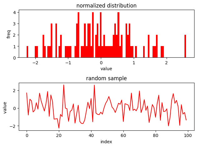
In [18]:
# 创建子图
fig, axs = plt.subplots(2,1)

# 填充数据、绘制图形
axs[0].hist(data, bins=100, color='red')
axs[1].plot(data, color='red')

# 参数设置
axs[0].set_title('normalized distribution')
axs[1].set_title('random sample')
axs[0].set_xlabel('value')
axs[0].set_ylabel('freq')
axs[1].set_xlabel('index')
axs[1].set_ylabel('value ')

# 调整子图距离
fig.tight_layout()

# 显示
plt.show()