SSD目标检测模型的实现
@
一、SSD模型的介绍
SSD: Single Shot MultiBox Detector one-stage目标检测模型
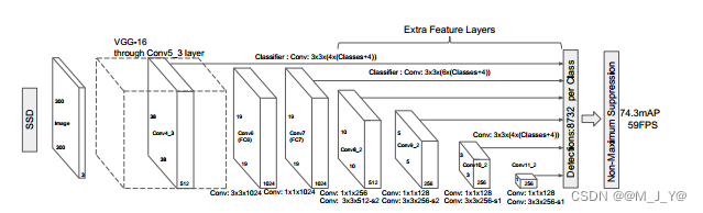
1. SSD模型的主干网络
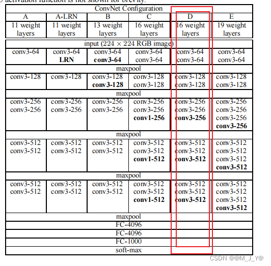
采用VGG网络模块,并进行一些改进:
将VGG16的FC6层和FC7层转变为卷积层,去除所有的Dropout层的FC8层,新增加Conv8层、Conv9层、Conv10层、Conv11层。
原VGG16模型如下
2.SSD采用的特征层
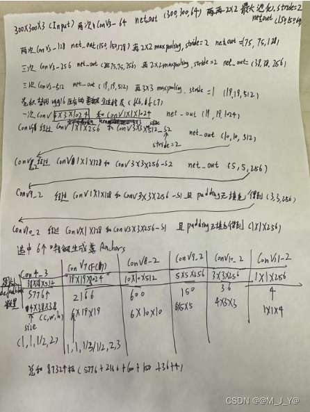
SSD模型采用的特征图为:
Conv4的第三次卷积的特征:38X38X512
Conv7卷积的特征:19X19X1024
Conv8的第二次卷积的特征:10X10X512
Conv9的第二次卷积的特征:5X5X256
Conv10的第二次卷积的特征:3X3X256
Conv11的第二次卷积的特征:1X1X256
SSD模型采用的有效特征层共6个,用于进行检测框的预测和目标分类。对应每张特征图的每个特征点生成anchors,每个特征层中的每个特征点对应的先验框数量为{4,6,6,6,4,4}。
3.SSD300(特征提取流程)
二、VOC格式数据集的准备
1.Voc数据集的存放方式为:
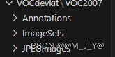
Annotations存放每张图片的XML文件,XML文件中图片的object信息表示这张图片所对应的目标检测框位置及其类别名称,每个图片可能会包含多个object。difficult表示识别难度。bndbox包含图片对应目标的位置信息(xmin,ymin,xmax,ymax)。size包含图片的宽、高和深度。name表示目标的类型名称。
XML文件包含的信息为:
<annotation>
	<folder>VOC2007</folder>
	<filename>000001.jpg</filename>
	<source>
		<database>The VOC2007 Database</database>
		<annotation>PASCAL VOC2007</annotation>
		<image>flickr</image>
		<flickrid>341012865</flickrid>
	</source>
	<owner>
		<flickrid>Fried Camels</flickrid>
		<name>Jinky the Fruit Bat</name>
	</owner>
	<size>
		<width>353</width>
		<height>500</height>
		<depth>3</depth>
	</size>
	<segmented>0</segmented>
	<object>
		<name>dog</name>
		<pose>Left</pose>
		<truncated>1</truncated>
		<difficult>0</difficult>
		<bndbox>
			<xmin>48</xmin>
			<ymin>240</ymin>
			<xmax>195</xmax>
			<ymax>371</ymax>
		</bndbox>
	</object>
	<object>
		<name>person</name>
		<pose>Left</pose>
		<truncated>1</truncated>
		<difficult>0</difficult>
		<bndbox>
			<xmin>8</xmin>
			<ymin>12</ymin>
			<xmax>352</xmax>
			<ymax>498</ymax>
		</bndbox>
	</object>
</annotation>
ImageSets的Main文件则是存放划分的训练集、验证集、测试集的文件索引信息文件,每个索引对应着图片的文件名称。
JPEGImages则用于存放原始图片。
2.Voc数据集的类别
Voc数据集的有20个小类,这里使用到的如下
aeroplane
bicycle
bird
boat
bottle
bus
car
cat
chair
cow
diningtable
dog
horse
motorbike
person
pottedplant
sheep
sofa
train
tvmonitor
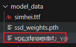
将这二十个小类保存到model_data文件夹下
3.训练集和验证集的准备
数据集的准备工作是生成用于训练的2007_train.txt和2007_val.txt文件,该文件每行对应一张图片,且包含了图片的图片路径及其目标框的位置、类别,如:
C:\Users\mjy\Desktop\ssd\VOCdevkit/VOC2007/JPEGImages/000005.jpg 263,211,324,339,8 165,264,253,372,8 241,194,295,299,8
C:\Users\mjy\Desktop\ssd\VOCdevkit/VOC2007/JPEGImages/000005.jpg是图片的保存路径。263,211,324,339,8 前面四个分别是目标框的位置(xmin,ymin,xmax,ymax)最后一个是目标的类别。
用于生成的代码如下:
import os
import random
import xml.etree.ElementTree as ET
import numpy as np
from utils.utils import get_classes
#   annotation_mode用于指定该文件运行时计算的内容
#   annotation_mode为2代表获得训练用的2007_train.txt、2007_val.txt
annotation_mode     = 2
classes_path        = 'model_data/voc_classes.txt'
#   指向VOC数据集所在的文件夹
#   默认指向根目录下的VOC数据集
VOCdevkit_path  = 'VOCdevkit'
VOCdevkit_sets  = [('2007', 'train'), ('2007', 'val')]
#获得class的名称和数量
classes, _      = get_classes(classes_path)
#获得图片的数量
photo_nums  = np.zeros(len(VOCdevkit_sets))
#获得类别的数量
nums        = np.zeros(len(classes))
def convert_annotation(year, image_id, list_file):
    #year=2007
    #image_id=000001
    in_file = open(os.path.join(VOCdevkit_path, 'VOC%s/Annotations/%s.xml'%(year, image_id)), encoding='utf-8')#打开xml文件
    tree=ET.parse(in_file)#解析xml文件
    root = tree.getroot()#获得根节点
    for obj in root.iter('object'):#遍历根节点下的object节点
        difficult = 0 #默认为0
        if obj.find('difficult')!=None:#如果object节点下有difficult节点
            difficult = obj.find('difficult').text#获得difficult节点的值
            #difficult 节点为1时,代表目标难以识别,为0时则相反。
            #在VOC数据集中,目标较小或者遮挡严重的标注为difficult。
        cls = obj.find('name').text#获得object节点下的name节点的值
        if cls not in classes or int(difficult)==1:#如果name节点的值不在classes中或者difficult节点的值为1
            continue
        cls_id = classes.index(cls)#获得name节点的值在classes中的索引
        xmlbox = obj.find('bndbox')#获得object节点下的bndbox节点
        b = (int(float(xmlbox.find('xmin').text)), int(float(xmlbox.find('ymin').text)), int(float(xmlbox.find('xmax').text)), int(float(xmlbox.find('ymax').text)))
        # b为目标的左上角和右下角坐标
        list_file.write(" " + ",".join([str(a) for a in b]) + ',' + str(cls_id))#将目标的坐标和类别写入list_file 前四个为坐标,最后一个为类别
        nums[classes.index(cls)] = nums[classes.index(cls)] + 1 #统计每个类别的数量

if __name__ == "__main__":
    random.seed(0)
    if " " in os.path.abspath(VOCdevkit_path):
        raise ValueError("数据集存放的文件夹路径与图片名称中不可以存在空格,否则会影响正常的模型训练,请注意修改。")
    print("Generate 2007_train.txt and 2007_val.txt for train.")
    type_index = 0#用于记录是2007_train.txt还是2007_val.txt
    for year, image_set in VOCdevkit_sets:#遍历VOCdevkit_sets
        image_ids = open(os.path.join(VOCdevkit_path, 'VOC%s/ImageSets/Main/%s.txt'%(year, image_set)), encoding='utf-8').read().strip().split()
        #打开对应的txt文件,获得图片的id 从测试集或者训练集中获得
        list_file = open('%s_%s.txt'%(year, image_set), 'w', encoding='utf-8')
        #打开对应的txt文件,用于写入图片的路径和标签 2007_train.txt或者2007_val.txt
        for image_id in image_ids:
            list_file.write('%s/VOC%s/JPEGImages/%s.jpg'%(os.path.abspath(VOCdevkit_path), year, image_id))#将图片的路径写入list_file
            convert_annotation(year, image_id, list_file)#将图片的路径和目标位置,标签写入list_file
            # list_file每行的内容为图片的路径和目标位置,标签
            list_file.write('\n')
        photo_nums[type_index] = len(image_ids)#统计图片的数量
        type_index += 1
        list_file.close()
    print("Generate 2007_train.txt and 2007_val.txt for train done.")
    def printTable(List1, List2):
        for i in range(len(List1[0])):
            print("|", end=' ')
            for j in range(len(List1)):
                print(List1[j][i].rjust(int(List2[j])), end=' ')#rjust() 方法返回一个原字符串右对齐,并使用空格填充至长度 width 的新字符串。
                print("|", end=' ')
            print()

    str_nums = [str(int(x)) for x in nums]#将nums中的数字转换为字符串
    #nums保存的是每个类别的数量
    #str_nums保存的是每个类别的数量的字符串形式
    tableData = [
        classes, str_nums
    ]#tableData为二维数组,第一行为类别,第二行为类别的数量
    #tableData的shape为(2,20)
    colWidths = [0]*len(tableData)#colWidths为一维数组,长度为tableData的长度,每个元素为0
    # colwidths的shape为(2,)
    len1 = 0
    for i in range(len(tableData)):
        for j in range(len(tableData[i])):
            if len(tableData[i][j]) > colWidths[i]:
                #如果tableData[i][j]的长度大于colWidths[i]
                #则将colWidths[i]的值改为tableData[i][j]的长度
                #colWidths[i]的值为tableData[i]中最长的字符串的长度
                colWidths[i] = len(tableData[i][j])
    printTable(tableData, colWidths)
    if photo_nums[0] <= 500:
        print("训练集数量小于500,属于较小的数据量,请注意设置较大的训练世代(Epoch)以满足足够的梯度下降次数(Step)。")
    if np.sum(nums) == 0:
        print("在数据集中并未获得任何目标,请注意修改classes_path对应自己的数据集,并且保证标签名字正确,否则训练将会没有任何效果!")
二、训练
1、模型的初始化
设置预训练模型路径,类别文件路径,输入图片的shape,anchors_size的大小,主干网络,学习率初始值,优化的方式,训练集路径,验证集路径。
具体设置如下
    Cuda = True#是否使用GPU
    seed            = 11#随机种子
    fp16            = False#是否使用fp16半精度训练
    classes_path    = 'model_data/voc_classes.txt'#类别文件的路径
    model_path      = 'model_data/ssd_weights.pth'#预训练权重的路径
    input_shape     = [300, 300]#输入图片的大小
    backbone        = "vgg"#主干特征提取网络的类型
    pretrained      = False#是否使用预训练权重(model_path不为空则pretrained的值无效)
    anchors_size    = [30, 60, 111, 162, 213, 264, 315]
    #anchor的大小根据voc数据集设定的,大多数情况下都是通用的。如果想要检测小物体,
    #可以修改anchors_size,一般调小浅层先验框的大小就行。因为浅层负责小物体检测!
    Init_Epoch          = 0
    UnFreeze_Epoch      = 200#总训练世代
    Unfreeze_batch_size = 8#解冻训练的batch_size
    Freeze_Train        = False #是否进行冻结训练
    Init_lr             = 2e-3 #模型的最大学习率
    Min_lr              = Init_lr * 0.01#模型的最小学习率,默认为最大学习率的0.01
    optimizer_type      = "sgd" # 当使用SGD优化器时建议设置   Init_lr=2e-3
    momentum            = 0.937#优化器内部使用到的momentum参数
    weight_decay        = 5e-4#权值衰减,可防止过拟合
    lr_decay_type       = 'cos'#学习率衰减策略
    save_period         = 10#多少个epoch保存一次权值
    save_dir            = 'logs'#权值保存的路径
    eval_flag           = True #是否进行评估
    eval_period         = 10 #多少个epoch评估一次
    num_workers         = 4 #多线程读取数据所使用的线程数
    train_annotation_path   = '2007_train.txt' #训练集的路径  训练图片路径和标签
    val_annotation_path     = '2007_val.txt' #验证集的路径 验证图片路径和标签
    seed_everything(seed)#设置随机种子
    ngpus_per_node  = torch.cuda.device_count() #GPU数量
    print("Use %d GPUs for training"%(ngpus_per_node)) #打印GPU数量
    device          = torch.device('cuda' if torch.cuda.is_available() else 'cpu') #使用GPU还是CPU
    local_rank      = 0#默认为0
    rank            = 0#默认为0
2.获取类的信息
Voc数据的类算上背景类一共21个类别。
    #1.获取类
    class_names, num_classes = get_classes(classes_path)#获取类别和类别数量
    num_classes += 1 #类别数量加1 再加上背景类,一共是num_classes+1类
3.生成anchors(default box)
为此后要训练的6张特征图生成anchors,一共8732个。通过计算将要产生的特征图的大小并为它们生成不同大小的anchors。anchors的shape为(8732,4)。对于每个特征层(feature map)上的每个特征点,将其中点作为中心,生成一系列同心的default box。对于每个特征层来说,根据其对应的aspect_ratio,会有两个正方形及不等的长方形。当ratio个数等于4时[1,1,1/2,2],6时[1,1,1/2,1/3,2,3]。
default box边长的计算方式为:
Scale的计算公式Smin=0.2,Smax=0.9

宽为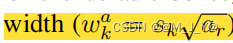
高为
我们当ratio =1时再添加一组的正方形
根据公式我们可以得到anchor的size,但是ratio=1时会添加新的一组大小组合(sqrt(sksk+1))。这时候我们的anchor_size需要多添加一个anchorsize。这里我们设置为7个。
anchors_size = [30, 60, 111, 162, 213, 264, 315]。default的边长实际计算如下:
规定default box的边长为anchors_size = [30, 60, 111, 162, 213, 264, 315]
对于6种特征层,会有6种不同的[min_size, max_size]的组合。
那么, default box边长的计算方式为:
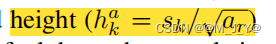
小正方形的边长为: \(min\_size\)
大正方形的边长为:\({\sqrt{min\_size \times max\_size}}\)
长方形框(ratio=1/2,1/3,2,3时)的Weight为:\(\frac{1}{\sqrt{aspect\_ratio}} \times min\_size\)
长方形框的Height为:\(\sqrt{aspect\_ratio} \times min\_size\)
核心代码如下
        for ar in self.aspect_ratios:
            # 首先添加一个较小的正方形
            if ar == 1 and len(box_widths) == 0:
                box_widths.append(self.min_size)
                box_heights.append(self.min_size)
            # 然后添加一个较大的正方形
            elif ar == 1 and len(box_widths) > 0:
                box_widths.append(np.sqrt(self.min_size * self.max_size))
                box_heights.append(np.sqrt(self.min_size * self.max_size))
            # 然后添加长方形
            elif ar != 1:
                box_widths.append(self.min_size * np.sqrt(ar))
                box_heights.append(self.min_size / np.sqrt(ar))
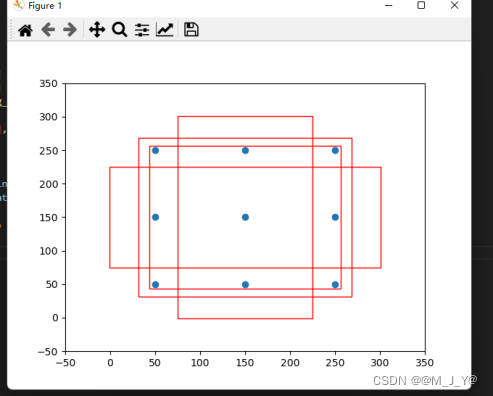
可视化一个3X3特征层的一个anchors如图所示。3X3特征层有四种长宽比。
详细代码如下
import numpy as np


class AnchorBox():
    def __init__(self, input_shape, min_size, max_size=None, aspect_ratios=None, flip=True):
        #特征图的大小
        self.input_shape = input_shape
        #最小的先验框的大小
        self.min_size = min_size
        #最大的先验框的大小
        self.max_size = max_size

        self.aspect_ratios = []
        # 将输入的1,2转换为[1, 1, 2, 1/2] 1,2,3转换为[1, 1, 2, 1/2, 3, 1/3]
        for ar in aspect_ratios:
            self.aspect_ratios.append(ar)
            self.aspect_ratios.append(1.0 / ar)

    def call(self, layer_shape, mask=None):
        # --------------------------------- #
        #   获取输入进来的特征层的宽和高
        #   比如38x38
        # --------------------------------- #
        layer_height    = layer_shape[0]
        layer_width     = layer_shape[1]
        # --------------------------------- #
        #   获取输入进来的图片的宽和高
        #   比如300x300
        # --------------------------------- #
        img_height  = self.input_shape[0]
        img_width   = self.input_shape[1]

        box_widths  = []
        box_heights = []
        # --------------------------------- #
        #   self.aspect_ratios一般有两个值
        #   [1, 1, 2, 1/2]
        #   [1, 1, 2, 1/2, 3, 1/3]
        # --------------------------------- #
        # 更加公式计算出来的宽高

        for ar in self.aspect_ratios:
            # 首先添加一个较小的正方形
            if ar == 1 and len(box_widths) == 0:
                box_widths.append(self.min_size)
                box_heights.append(self.min_size)
            # 然后添加一个较大的正方形
            elif ar == 1 and len(box_widths) > 0:
                box_widths.append(np.sqrt(self.min_size * self.max_size))
                box_heights.append(np.sqrt(self.min_size * self.max_size))
            # 然后添加长方形
            elif ar != 1:
                box_widths.append(self.min_size * np.sqrt(ar))
                box_heights.append(self.min_size / np.sqrt(ar))

        # --------------------------------- #
        #   获得所有先验框的宽高1/2
        # --------------------------------- #
        box_widths  = 0.5 * np.array(box_widths)
        box_heights = 0.5 * np.array(box_heights)

        # --------------------------------- #
        #   每一个特征层对应的步长 layer_width特征图的宽度
        #    原图到特征图的缩放比例
        # --------------------------------- #
        step_x = img_width / layer_width
        step_y = img_height / layer_height

        # --------------------------------- #
        #   生成网格中心
        # --------------------------------- #
        # np.linspace:这是NumPy库中的一个函数,用于生成等间距的数值序列。
        # 获取每个网格的中心点
        linx = np.linspace(0.5 * step_x, img_width - 0.5 * step_x,
                           layer_width)
        liny = np.linspace(0.5 * step_y, img_height - 0.5 * step_y,
                           layer_height)
        #得到二维网格
        centers_x, centers_y = np.meshgrid(linx, liny)
        #展平
        centers_x = centers_x.reshape(-1, 1)
        centers_y = centers_y.reshape(-1, 1)

        # 每一个先验框需要两个(centers_x, centers_y),前一个用来计算左上角,后一个计算右下角
        num_anchors_ = len(self.aspect_ratios)
        #anchor_boxes中每个元素表示当前所在锚框的中心坐标 x和y
        anchor_boxes = np.concatenate((centers_x, centers_y), axis=1)

        # 目前维度为 特征图像素的个数X2
        anchor_boxes = np.tile(anchor_boxes, (1, 2 * num_anchors_))

        # 获得先验框的左上角和右下角 box_widths为一半的宽度 box_heights为一半的高度
        # xmin
        anchor_boxes[:, ::4]    -= box_widths
        #ymin
        anchor_boxes[:, 1::4]   -= box_heights
        #xmax
        anchor_boxes[:, 2::4]   += box_widths
        #ymax
        anchor_boxes[:, 3::4]   += box_heights

        # --------------------------------- #
        #   将先验框变成小数的形式
        #   归一化
        # --------------------------------- #
        #将xmin xmax 归一化
        anchor_boxes[:, ::2]    /= img_width
        #将ymin ymax 归一化
        anchor_boxes[:, 1::2]   /= img_height
        # 当前维度为 (特征图像素Xnum_anchors)X 4 4是xmin ymin xmax ymax
        anchor_boxes = anchor_boxes.reshape(-1, 4)

        # 进行一个clap 防止值超出0 或者1之间
        # min max 用于限制范围
        # minimum 用于限制最小值 按位置比较两个数组的元素,并返回最小值
        # maximum 用于限制最大值 按位置比较两个数组的元素,并返回最大值
        anchor_boxes = np.minimum(np.maximum(anchor_boxes, 0.0), 1.0)

        return anchor_boxes

#---------------------------------------------------#
#   用于计算共享特征层的大小
#---------------------------------------------------#
def get_vgg_output_length(height, width):
    #8次卷积 5次池化 后面三次卷积不进行池化 第6次设置步长为2 后面两次步长为1但不填充
    filter_sizes    = [3, 3, 3, 3, 3, 3, 3, 3]
    padding         = [1, 1, 1, 1, 1, 1, 0, 0]
    stride          = [2, 2, 2, 2, 2, 2, 1, 1]
    feature_heights = []
    feature_widths  = []

    for i in range(len(filter_sizes)):
        # 300x300 -> 150x150 -> 75x75 -> 38x38 -> 19x19 -> 10x10 -> 5x5 -> 3x3
        # 高的计算方式为 (height + 2*padding - filter_size) // stride + 1
        # 宽的计算方式为 (width + 2*padding - filter_size) // stride + 1
        height  = (height + 2*padding[i] - filter_sizes[i]) // stride[i] + 1
        width   = (width + 2*padding[i] - filter_sizes[i]) // stride[i] + 1
        feature_heights.append(height)
        feature_widths.append(width)
    #取最后六个特征层的大小
    return np.array(feature_heights)[-6:], np.array(feature_widths)[-6:]

# 输入图像的大小为300x300 anchors_size 有7个
def get_anchors(input_shape = [300,300], anchors_size = [30, 60, 111, 162, 213, 264, 315]):

    # 获得每个特征层的大小
    feature_heights, feature_widths = get_vgg_output_length(input_shape[0], input_shape[1])
    #宽高比为 1, 1, 2, 1/2, 3, 1/3
    aspect_ratios = [[1, 2], [1, 2, 3], [1, 2, 3], [1, 2, 3], [1, 2], [1, 2]]
    anchors = []

    for i in range(len(feature_heights)):
        #先初始化一个AnchorBox类在调用生成先验框
        anchor_boxes = AnchorBox(input_shape, anchors_size[i], max_size = anchors_size[i+1],
                    aspect_ratios = aspect_ratios[i]).call([feature_heights[i], feature_widths[i]])
        anchors.append(anchor_boxes)
    # 将所有的先验框进行堆叠
    #按照列方向进行堆叠
    #anchors大小为 8732X4
    anchors = np.concatenate(anchors, axis=0)
    return anchors
4.获取模型
加载预训练的权重
 model = SSD300(num_classes, backbone, pretrained)#实例化模型
    weights_init(model)#初始化模型权重
 if model_path != '':
        if local_rank == 0:
            print('Load weights {}.'.format(model_path))
        model_dict      = model.state_dict() #model_dict是模型权重
        pretrained_dict = torch.load(model_path, map_location = device) #pretrained_dict 是预训练权重
        load_key, no_load_key, temp_dict = [], [], {}

        for k, v in pretrained_dict.items():
            if k in model_dict.keys() and np.shape(model_dict[k]) == np.shape(v):#如果预训练权重的key在模型权重中,且形状相同
                temp_dict[k] = v#将预训练权重的键值对存入temp_dict
                load_key.append(k)#将预训练权重的键存入load_key
            else:
                no_load_key.append(k)#如果预训练权重的key不在在模型权重且形状不相同,将预训练权重的键存入no_load_key
        model_dict.update(temp_dict)#update是将temp_dict中的键值对更新到model_dict中
        model.load_state_dict(model_dict)#加载权重
        #  显示没有匹配上的Key
        if local_rank == 0:
            print("\nSuccessful Load Key:", str(load_key)[:500], "……\nSuccessful Load Key Num:", len(load_key))
            print("\nFail To Load Key:", str(no_load_key)[:500], "……\nFail To Load Key num:", len(no_load_key))
            print("\n\033[1;33;44m温馨提示,head部分没有载入是正常现象,Backbone部分没有载入是错误的。\033[0m")
vgg 主干网络定义如下
import torch.nn as nn
from torch.hub import load_state_dict_from_url


'''
该代码用于获得VGG主干特征提取网络的输出。
输入变量i代表的是输入图片的通道数,通常为3。

300, 300, 3 -> 300, 300, 64 -> 300, 300, 64 -> 150, 150, 64 -> 150, 150, 128 -> 150, 150, 128 -> 75, 75, 128 ->
75, 75, 256 -> 75, 75, 256 -> 75, 75, 256 -> 38, 38, 256 -> 38, 38, 512 -> 38, 38, 512 -> 38, 38, 512 -> 19, 19, 512 ->
19, 19, 512 -> 19, 19, 512 -> 19, 19, 512 -> 19, 19, 512 -> 19, 19, 1024 -> 19, 19, 1024

38, 38, 512的序号是22
19, 19, 1024的序号是34
'''
base = [64, 64, 'M', 128, 128, 'M', 256, 256, 256, 'C', 512, 512, 512, 'M',
            512, 512, 512]

def vgg(pretrained = False):
    layers = []
    in_channels = 3
    for v in base:
        if v == 'M':
            layers += [nn.MaxPool2d(kernel_size=2, stride=2)]
        elif v == 'C':
            layers += [nn.MaxPool2d(kernel_size=2, stride=2, ceil_mode=True)]
        else:
            conv2d = nn.Conv2d(in_channels, v, kernel_size=3, padding=1)
            layers += [conv2d, nn.ReLU(inplace=True)]
            in_channels = v
    # 19, 19, 512 -> 19, 19, 512
    pool5 = nn.MaxPool2d(kernel_size=3, stride=1, padding=1)
    # 19, 19, 512 -> 19, 19, 1024
    conv6 = nn.Conv2d(512, 1024, kernel_size=3, padding=6, dilation=6)
    # 19, 19, 1024 -> 19, 19, 1024
    conv7 = nn.Conv2d(1024, 1024, kernel_size=1)
    layers += [pool5, conv6,
               nn.ReLU(inplace=True), conv7, nn.ReLU(inplace=True)]

    model = nn.ModuleList(layers)

    if pretrained:
        # 加载预训练模型
        state_dict = load_state_dict_from_url("https://download.pytorch.org/models/vgg16-397923af.pth", model_dir="./model_data")
        # 去掉features.
        state_dict = {k.replace('features.', '') : v for k, v in state_dict.items()}
        # 加载权重 strict = False表示不严格匹配
        model.load_state_dict(state_dict, strict = False)
    return model

if __name__ == "__main__":
    net = vgg()
    for i, layer in enumerate(net):
        print(i, layer)
SSD300的模型定义如下
class SSD300(nn.Module):
    def __init__(self, num_classes, backbone_name, pretrained = False):
        super(SSD300, self).__init__()
        self.num_classes    = num_classes
        if backbone_name    == "vgg":
            self.vgg        = add_vgg(pretrained)
            self.extras     = add_extras(1024, backbone_name)
            self.L2Norm     = L2Norm(512, 20)
            mbox            = [4, 6, 6, 6, 4, 4]
            loc_layers      = []
            conf_layers     = []
            #Conv4_3 在第21层
            #FC6 在倒数第二层 最后一层是Relu
            backbone_source = [21, -2]
            #---------------------------------------------------#
            #   在add_vgg获得的特征层里
            #   第21层和-2层可以用来进行回归预测和分类预测。
            #   分别是conv4-3(38,38,512)和conv7(19,19,1024)的输出
            #---------------------------------------------------#
            for k, v in enumerate(backbone_source):
                loc_layers  += [nn.Conv2d(self.vgg[v].out_channels, mbox[k] * 4, kernel_size = 3, padding = 1)]
                conf_layers += [nn.Conv2d(self.vgg[v].out_channels, mbox[k] * num_classes, kernel_size = 3, padding = 1)]
            #-------------------------------------------------------------#
            #   在add_extras获得的特征层里
            #   第1层、第3层、第5层、第7层可以用来进行回归预测和分类预测。
            #   shape分别为(10,10,512), (5,5,256), (3,3,256), (1,1,256)
            #-------------------------------------------------------------#
            for k, v in enumerate(self.extras[1::2], 2):
                loc_layers  += [nn.Conv2d(v.out_channels, mbox[k] * 4, kernel_size = 3, padding = 1)]
                conf_layers += [nn.Conv2d(v.out_channels, mbox[k] * num_classes, kernel_size = 3, padding = 1)]


            #defaultbox 数量 每个特征图对应的每个特征点拥有的default box 个数
            mbox            = [4, 6, 6, 6, 4, 4]

            loc_layers      = []
            conf_layers     = []
            out_channels    = [512, 1024]
            #---------------------------------------------------#
            #   在add_vgg获得的特征层里
            #   第layer3层和layer4层可以用来进行回归预测和分类预测。
            #---------------------------------------------------#
            for k, v in enumerate(out_channels):
                loc_layers  += [nn.Conv2d(out_channels[k], mbox[k] * 4, kernel_size = 3, padding = 1)]
                conf_layers += [nn.Conv2d(out_channels[k], mbox[k] * num_classes, kernel_size = 3, padding = 1)]
            #-------------------------------------------------------------#
            #   在add_extras获得的特征层里
            #   第1层、第3层、第5层、第7层可以用来进行回归预测和分类预测。
            #   shape分别为(10,10,512), (5,5,256), (3,3,256), (1,1,256)
            #-------------------------------------------------------------#
            for k, v in enumerate(self.extras[1::2], 2):
                loc_layers  += [nn.Conv2d(v.out_channels, mbox[k] * 4, kernel_size = 3, padding = 1)]
                conf_layers += [nn.Conv2d(v.out_channels, mbox[k] * num_classes, kernel_size = 3, padding = 1)]
        else:
            raise ValueError("The backbone_name is not support")

        #loc_layers/conf_layers 参数为(通道数,每个特征点对应的defaultbox 数量,卷积核的大小,填充)
        self.loc            = nn.ModuleList(loc_layers)
        self.conf           = nn.ModuleList(conf_layers)
        #主干名为backbone
        self.backbone_name  = backbone_name
    #torch.Size([2, 3, 300, 300])
    #x (batch_size, input_channels, input_height, input_width)
    def forward(self, x):
        #---------------------------#
        #   x是300,300,3
        #---------------------------#
        sources = list()
        loc     = list()
        conf    = list()

        #---------------------------#
        #   获得conv4_3的内容
        #   shape为38,38,512
        #---------------------------#
        if self.backbone_name == "vgg":
            for k in range(23):
                x= self.vgg[k](x)

        #---------------------------#
        #   conv4_3的内容
        #   需要进行L2标准化
        #---------------------------#
        s = self.L2Norm(x)
        sources.append(s)
        #soures 中单个元素值为 (输入通道数,输出通道数,卷积核大小,padding填充)
        #---------------------------#
        #   获得conv7的内容
        #   shape为19,19,1024
        #---------------------------#
        if self.backbone_name == "vgg":
            for k in range(23, len(self.vgg)):
                x = self.vgg[k](x)

        sources.append(x)
        #-------------------------------------------------------------#
        #   在add_extras获得的特征层里
        #   第1层、第3层、第5层、第7层可以用来进行回归预测和分类预测。
        #   shape分别为(10,10,512), (5,5,256), (3,3,256), (1,1,256)
        #-------------------------------------------------------------#
        for k, v in enumerate(self.extras):
            x = F.relu(v(x), inplace=True)
            if self.backbone_name == "vgg" :
                if k % 2 == 1:
                    sources.append(x)
            else:
                sources.append(x)

        #-------------------------------------------------------------#
        #   为获得的6个有效特征层添加回归预测和分类预测
        #-------------------------------------------------------------#
        #  l 是 loc 回归层 c 是分类层
        # l/c(通道数,每个特征点对应的defaultbox 数量,卷积核的大小,填充)
        # x 是source 获得6个特征层
        # loc[0] (16X38X38X16)
        for (x, l, c) in zip(sources, self.loc, self.conf):
            loc.append(l(x).permute(0, 2, 3, 1).contiguous())
            conf.append(c(x).permute(0, 2, 3, 1).contiguous())
        #loc 现在的值(batch_size, height, width,channels)
        # 其中channel 用作回归预测  大小为 defaultbox * 4(4是四个坐标)
        # conf 其中channel 用作回归预测  大小为 defaultbox * classnum(类的数量)
        '''
        将维度从 (batch_size, channels, height, width) 重新排列为 (batch_size, height, width, channels)。
        这通常是因为在目标检测的常见表示中,最后一个维度通常表示不同的类别的预测。
        '''

        #-------------------------------------------------------------#
        #   进行reshape方便堆叠
        #-------------------------------------------------------------#

        loc     = torch.cat([o.view(o.size(0), -1) for o in loc], 1)
        conf    = torch.cat([o.view(o.size(0), -1) for o in conf], 1)

        #-------------------------------------------------------------#
        #   loc会reshape到batch_size, num_anchors, 4 xywh
        #   conf会reshap到batch_size, num_anchors, self.num_classes
        #-------------------------------------------------------------#
        output = (
            loc.view(loc.size(0), -1, 4),
            conf.view(conf.size(0), -1, self.num_classes),
        )
        return output
模型的输出有两个值一个conf(类别信息shape为8732Xnum_classes) 一个loc(8732X4)
5. 得到损失函数(包括了hard example mining)
criterion = MultiboxLoss(num_classes, neg_pos_ratio=3.0)# 获得损失函数
SSD模型针对包含多个的目标的图片进行处理,其损失函数包括两部分:置信度损失和位置损失,计算方式为:
\(L(x,c,l,g)= \frac{1}N[L_conf(x,c)+αL_loc(x,l,g)]\)
c, l, g 分别表示为类别置信度预测值、预测框和真实框的参数(宽高和中心位置)
N表示正样本的数量
\(x_{ij}^{p}=\{1,0\}\),1表示第i个default box和类别为p的第j的gt box相匹配;0表示未匹配。
\(L_conf\) 和\(L_loc\) 分别表示置信度损失和位置损失。
位置损失采用\(smooth_{L1} Loss\),该损失是计算需要回归至default bounding box 的中心及宽度、高度的偏移量,其计算方式为:
\(l_i^m,g_j^m\)分别表示第i个预测框和调整的第j个gt box 的中心、宽和高。
置信度损失采用多个类别上的softmax损失:
前向传播过程(包括了hard example mining)
1.计算分类的loss y_true[:, :, 4:-1]表示取y_true的第4个维度到倒数第二个维度 5-24 y_pred[:, :, 4:]表示取y_pred的第4个维度到最后一个维度 4-24
2.计算框的位置的loss y_true[:, :, :4]表示取y_true的第一个维度到第四个维度 0-3 y_pred[:, :, :4]表示取y_pred的第一个维度到第四个维度 0-3
3.获取所有的正标签loc loss y_true[:, :, -1]表示取y_true的最后一个维度 -1
4.获取所有的正标签分类loss y_true[:, :, -1]表示取y_true的最后一个维度 -1
5.每一张图的正样本的个数 即每个batch中每张图的正样本的数量
6.每一张图的负样本的个数 取剩余的框的数量减去正样本的数量和neg_pos_ratio(3)倍数的正样本数量的最小值
7.pos_num_neg_mask shape是torch.Size([2, 8732]) 代表每张图的负样本的数量是否大于0
8.求整个batch应该的负样本数量总和 如果所有的图,正样本的数量均为0 那么则默认选取100个先验框作为负样本
9.只有没有包含物体的先验框才得到保留 这就是实际上不包含物体的anchors的所有种类预测概率求和
10.选取的前100个难分类样本的分类loss
11.正样本的分类loss + 负样本的分类loss + alpha * 正样本的框的位置loss (负样本取的数量为neg_pos_ratio倍的正样本)
具体代码如下
class MultiboxLoss(nn.Module):

    def __init__(self, num_classes, alpha=1.0, neg_pos_ratio=3.0,
                 background_label_id=0, negatives_for_hard=100.0):
        #当前的类别数量
        self.num_classes = num_classes
        #alpha是用来控制置信度损失的比重 loss = L_conf + alpha * L_loc 根据论文指出根据交叉验证计算出来1.0比较合适
        self.alpha = alpha
        #负正样本比例 3:1
        self.neg_pos_ratio = neg_pos_ratio
        #背景类别的id
        if background_label_id != 0:
            raise Exception('Only 0 as background label id is supported')
        #负样本的数量
        self.background_label_id = background_label_id
        #每张图片的负样本数量 100

        self.negatives_for_hard = torch.FloatTensor([negatives_for_hard])[0]
        # negatives_for_hard 的shape是torch.Size([1]),所以要加[0]变成torch.Size([])


    def _l1_smooth_loss(self, y_true, y_pred):
        # 计算预测值和真实值的差值
        abs_loss = torch.abs(y_true - y_pred)
        # 绝对值 小于1的部分使用0.5x^2作为loss,大于1的部分使用|x|-0.5作为loss
        sq_loss = 0.5 * (y_true - y_pred)**2

        #使用where函数,如果abs_loss小于1,那么使用sq_loss,否则使用abs_loss-0.5作为loss
        l1_loss = torch.where(abs_loss < 1.0, sq_loss, abs_loss - 0.5)
        # 将每个框的loss相加
        return torch.sum(l1_loss, -1)

    def _softmax_loss(self, y_true, y_pred):
        # 计算softmax的loss
        # y_pred的值域是[0,1],但是由于log函数的特性,我们需要将y_pred的值域变成[1e-7,1]
        # clamp函数的作用就是将y_pred的值域限制在[1e-7,1]
        # clamp参数min表示最小值,max表示最大值 限制最小值为1e-7
        y_pred = torch.clamp(y_pred, min = 1e-7)
        # torch.log(y_pred)表示求y_pred的自然对数
        # 对所有的类别求和
        # y_true * torch.log(y_pred)表示将y_true中为1的部分保留下来,为0的部分变成0
        # torch.sum(y_true * torch.log(y_pred),axis=-1)表示对最后一维求和

        # y_true=0表示背景类别,y_true=1表示正样本
        softmax_loss = -torch.sum(y_true * torch.log(y_pred),
                                      axis=-1)
        return softmax_loss

    def forward(self, y_true, y_pred):
        # --------------------------------------------- #
        #   y_true batch_size, 8732, 4 + self.num_classes + 1
        #   y_pred batch_size, 8732, 4 + self.num_classes
        # --------------------------------------------- #


        num_boxes       = y_true.size()[1]
        # numboxes是8732

        y_pred          = torch.cat([y_pred[0], nn.Softmax(-1)(y_pred[1])], dim = -1)
        # y_pred目前的shape为torch.Size([2, 8732, 25])
        #y_pred[0]是预测的框的位置,y_pred[1]是预测的框的类别
        #y_pred[0] shape是torch.Size([2, 8732, 4]),y_pred[1] shape是torch.Size([2, 8732, 21])
        '''
        y_pred[0] 是一个张量,假设它包含了模型的某些预测值。它是拼接操作的第一个输入张量。

        nn.Softmax(-1)(y_pred[1]) 是一个张量,它首先应用了 softmax 操作到 y_pred[1] 上,
        然后生成一个包含概率分布的张量。这是拼接操作的第二个输入张量。

        dim=-1 表示在最后一个维度上进行拼接,也就是列维度。这是拼接操作的维度参数。
        '''
        # --------------------------------------------- #
        #   分类的loss
        #   batch_size,8732,21 -> batch_size,8732
        # --------------------------------------------- #
        # 1.计算分类的loss y_true[:, :, 4:-1]表示取y_true的第4个维度到倒数第二个维度 5-24 y_pred[:, :, 4:]表示取y_pred的第4个维度到最后一个维度 4-24
        conf_loss = self._softmax_loss(y_true[:, :, 4:-1], y_pred[:, :, 4:])

        # --------------------------------------------- #
        #   框的位置的loss
        #   batch_size,8732,4 -> batch_size,8732
        # --------------------------------------------- #
        # 2.计算框的位置的loss y_true[:, :, :4]表示取y_true的第一个维度到第四个维度 0-3 y_pred[:, :, :4]表示取y_pred的第一个维度到第四个维度 0-3
        loc_loss = self._l1_smooth_loss(y_true[:, :, :4],
                                        y_pred[:, :, :4])

        # --------------------------------------------- #
        #   获取所有的正标签的loss
        # --------------------------------------------- #
        # 3.获取所有的正标签loc loss y_true[:, :, -1]表示取y_true的最后一个维度 -1
        # y_true[:, :, -1]表示是否包含物体
        pos_loc_loss = torch.sum(loc_loss * y_true[:, :, -1],
                                     axis=1)
        # 4.获取所有的正标签分类loss y_true[:, :, -1]表示取y_true的最后一个维度 -1
        # y_true[:, :, -1]表示是否包含物体
        pos_conf_loss = torch.sum(conf_loss * y_true[:, :, -1],
                                      axis=1)

        # --------------------------------------------- #
        #   每一张图的正样本的个数
        #   num_pos     [batch_size,]
        # --------------------------------------------- #
        # 5.每一张图的正样本的个数 即每个batch中每张图的正样本的数量
        num_pos = torch.sum(y_true[:, :, -1], axis=-1)

        # --------------------------------------------- #
        #   每一张图的负样本的个数
        #   num_neg     [batch_size,]
        # --------------------------------------------- #

        # 6.每一张图的负样本的个数  取剩余的框的数量减去正样本的数量和neg_pos_ratio(3)倍数的正样本数量的最小值
        num_neg = torch.min(self.neg_pos_ratio * num_pos, num_boxes - num_pos)

        # 7.pos_num_neg_mask shape是torch.Size([2, 8732]) 代表每张图的负样本的数量是否大于0
        pos_num_neg_mask = num_neg > 0
        # --------------------------------------------- #
        #   如果所有的图,正样本的数量均为0
        #   那么则默认选取100个先验框作为负样本
        # --------------------------------------------- #

        has_min = torch.sum(pos_num_neg_mask)

        # --------------------------------------------- #
        #   从这里往后,与视频中看到的代码有些许不同。
        #   由于以前的负样本选取方式存在一些问题,
        #   我对该部分代码进行重构。
        #   求整个batch应该的负样本数量总和
        # --------------------------------------------- #

        # 8.求整个batch应该的负样本数量总和 如果所有的图,正样本的数量均为0 那么则默认选取100个先验框作为负样本
        num_neg_batch = torch.sum(num_neg) if has_min > 0 else self.negatives_for_hard

        # --------------------------------------------- #
        #   对预测结果进行判断,如果该先验框没有包含物体
        #   那么它的不属于背景的预测概率过大的话
        #   就是难分类样本
        # --------------------------------------------- #
        confs_start = 4 + self.background_label_id + 1
        #background_label_id=0
        #confs_start=5 代表第5个维度开始是不属于背景的预测概率

        confs_end   = confs_start + self.num_classes - 1
        #confs_end=25 代表第25个维度结束是不属于背景的预测概率

        # --------------------------------------------- #
        #   batch_size,8732
        #   把不是背景的概率求和,求和后的概率越大
        #   代表越难分类。
        # --------------------------------------------- #
        max_confs = torch.sum(y_pred[:, :, confs_start:confs_end], dim=2)
        #y_pred[:, :, confs_start:confs_end]表示取y_pred的第5个维度到第25个维度 4-24
        #torch.sum(y_pred[:, :, confs_start:confs_end], dim=2)表示对第三个维度求和
        #max_confs shape是torch.Size([2, 8732]) 代表每张图的不属于背景的预测概率求和
        # max_confs大的话,代表越难分类 anchors就是难分类样本
        # --------------------------------------------------- #
        #   只有没有包含物体的先验框才得到保留
        #   我们在整个batch里面选取最难分类的num_neg_batch个
        #   先验框作为负样本。
        # --------------------------------------------------- #

        # 9.只有没有包含物体的先验框才得到保留 这就是实际上不包含物体的anchors的所有种类预测概率求和
        max_confs   = (max_confs * (1 - y_true[:, :, -1])).view([-1])
        #max_confs的shape是torch.Size([17464]) 代表所有的anchors的所有种类预测概率求和
        #y_true[:, :, -1]表示取y_true的最后一个维度 -1

        _, indices  = torch.topk(max_confs, k = int(num_neg_batch.cpu().numpy().tolist()))
        #indices shape是torch.Size([100]) 代表选取的100个难分类样本的索引
        #indices是max_confs中最大的100个值的索引

        neg_conf_loss = torch.gather(conf_loss.view([-1]), 0, indices)
        #neg_conf_loss shape是torch.Size([100]) 代表选取的100个难分类样本的分类loss
        #conf_loss.view([-1])表示将conf_loss的shape变成torch.Size([17464]) 代表所有的anchors的分类loss
        #indices表示选取的100个难分类样本的索引
        #torch.gather(conf_loss.view([-1]), 0, indices)表示选取的100个难分类样本的分类loss

        # 进行归一化
        num_pos     = torch.where(num_pos != 0, num_pos, torch.ones_like(num_pos))
        #num_pos shape是torch.Size([2]) 代表每张图的正样本的数量
        #torch.ones_like(num_pos)表示生成一个和num_pos相同shape的全1张量
        #torch.where(num_pos != 0, num_pos, torch.ones_like(num_pos))表示如果num_pos不等于0,那么就取num_pos,否则就取torch.ones_like(num_pos) 全一张量


        total_loss  = torch.sum(pos_conf_loss) + torch.sum(neg_conf_loss) + torch.sum(self.alpha * pos_loc_loss)
        #total_loss shape是torch.Size([]) 代表总的loss
        #torch.sum(pos_conf_loss)表示所有的正样本的分类loss相加
        # 正样本的分类loss + 负样本的分类loss + alpha * 正样本的框的位置loss (负样本取的数量为neg_pos_ratio倍的正样本)

        total_loss  = total_loss / torch.sum(num_pos)#torch.sum(num_pos)表示所有的正样本的数量相加
        return total_loss


# get_lr_scheduler函数用来获取学习率调整函数 余弦退火
def get_lr_scheduler(lr_decay_type, lr, min_lr, total_iters, warmup_iters_ratio = 0.05, warmup_lr_ratio = 0.1, no_aug_iter_ratio = 0.05, step_num = 10):
    def yolox_warm_cos_lr(lr, min_lr, total_iters, warmup_total_iters, warmup_lr_start, no_aug_iter, iters):
        if iters <= warmup_total_iters:
            lr = (lr - warmup_lr_start) * pow(iters / float(warmup_total_iters), 2) + warmup_lr_start
        elif iters >= total_iters - no_aug_iter:
            lr = min_lr
        else:
            lr = min_lr + 0.5 * (lr - min_lr) * (
                1.0 + math.cos(math.pi* (iters - warmup_total_iters) / (total_iters - warmup_total_iters - no_aug_iter))
            )
        return lr

    warmup_total_iters  = min(max(warmup_iters_ratio * total_iters, 1), 3)
    warmup_lr_start     = max(warmup_lr_ratio * lr, 1e-6)
    no_aug_iter         = min(max(no_aug_iter_ratio * total_iters, 1), 15)
    func = partial(yolox_warm_cos_lr ,lr, min_lr, total_iters, warmup_total_iters, warmup_lr_start, no_aug_iter)
    return func


#设置优化器的学习率
def set_optimizer_lr(optimizer, lr_scheduler_func, epoch):
    #根据epoch计算当前的学习率
    lr = lr_scheduler_func(epoch)
    #将学习率设置到optimizer中
    for param_group in optimizer.param_groups:
        param_group['lr'] = lr

def weights_init(net, init_type='normal', init_gain=0.02):
    def init_func(m):
        classname = m.__class__.__name__
        if hasattr(m, 'weight') and classname.find('Conv') != -1:
            if init_type == 'normal':
                torch.nn.init.normal_(m.weight.data, 0.0, init_gain)
            elif init_type == 'xavier':
                torch.nn.init.xavier_normal_(m.weight.data, gain=init_gain)
            elif init_type == 'kaiming':
                torch.nn.init.kaiming_normal_(m.weight.data, a=0, mode='fan_in')
            elif init_type == 'orthogonal':
                torch.nn.init.orthogonal_(m.weight.data, gain=init_gain)
            else:
                raise NotImplementedError('initialization method [%s] is not implemented' % init_type)
        elif classname.find('BatchNorm2d') != -1:
            torch.nn.init.normal_(m.weight.data, 1.0, 0.02)
            torch.nn.init.constant_(m.bias.data, 0.0)
    print('initialize network with %s type' % init_type)
    net.apply(init_func)
6. 读取训练集和验证集
代码如下
if Cuda:
 model_train = torch.nn.DataParallel(model)#多GPU训练
 cudnn.benchmark = True#设置为True,那么每次运行卷积神经网络的时候都会去寻找最适合当前配置的高效算法,来达到优化运行效率的问题。
 model_train = model_train.cuda()#将模型转为cuda模式
with open(train_annotation_path, encoding='utf-8') as f:#读取训练集的txt
 train_lines = f.readlines()
with open(val_annotation_path, encoding='utf-8') as f:#读取验证集的txt
 val_lines   = f.readlines()
num_train   = len(train_lines)#训练集的大小
num_val     = len(val_lines)  #验证集的大小
7.计算步长
计算总步长 判读是否达到建议的总步长
  wanted_step = 5e4 # 想要的总步长
        # 计算总步长 判读是否达到建议的总步长
        total_step  = num_train // Unfreeze_batch_size * UnFreeze_Epoch
        # Unfreeze_batch_size =8
        # UnFreeze_Epoch = 200

        if total_step <= wanted_step:
            if num_train // Unfreeze_batch_size == 0:
                raise ValueError('数据集过小,无法进行训练,请扩充数据集。')
            wanted_epoch = wanted_step // (num_train // Unfreeze_batch_size) + 1
            print("\n\033[1;33;44m[Warning] 使用%s优化器时,建议将训练总步长设置到%d以上。\033[0m"%(optimizer_type, wanted_step))
            print("\033[1;33;44m[Warning] 本次运行的总训练数据量为%d,Unfreeze_batch_size为%d,共训练%d个Epoch,计算出总训练步长为%d。\033[0m"%(num_train, Unfreeze_batch_size, UnFreeze_Epoch, total_step))
            print("\033[1;33;44m[Warning] 由于总训练步长为%d,小于建议总步长%d,建议设置总世代为%d。\033[0m"%(total_step, wanted_step, wanted_epoch))
8.调整学习率获得学习率的公式,SGD优化器
nbs             = 64
        lr_limit_max    = 5e-2
        lr_limit_min    = 5e-5
        Init_lr_fit     = min(max(batch_size / nbs * Init_lr, lr_limit_min), lr_limit_max) #INIT_LR = 2e-3 batch_size = 8
        #Init_lr_fit的值计算为:min(max(8/64*2e-3, 5e-5), 5e-2) = 2e-3 *(1/8)=0.00025
        Min_lr_fit      = min(max(batch_size / nbs * Min_lr, lr_limit_min * 1e-2), lr_limit_max * 1e-2) #MIN_LR = 2e-5 batch_size = 8
        #Min_lr_fit的值计算为 min(max(8/64*2e-5, 5e-5*1e-2), 5e-2) =  2.5e-6
        #10.SGD优化器
        optimizer = optim.SGD(model.parameters(), Init_lr_fit, momentum = momentum, nesterov=True, weight_decay = weight_decay)#选择优化器
        #11.获得学习率下降的公式
        lr_scheduler_func = get_lr_scheduler(lr_decay_type, Init_lr_fit, Min_lr_fit, UnFreeze_Epoch) #   获得学习率下降的公式
9.使用SSDDataset类实例化训练集和验证集的数据加载器(包括了添加灰度条进行resize和encode过程)
- 训练时进行数据的随机增强
验证时不进行数据的随机增强 - 对真实框进行处理
- 对box坐标归一化 并得到one_hot_label
- 为每个先验框分配真实框 使得每个先验框都有一个真实框与之对应 (通过best_iou_idx等操作)shape为num_anchors, 4 + num_classes + 1
>代码如下
```python
train_dataset   = SSDDataset(train_lines, input_shape, anchors, batch_size, num_classes, train = True)#训练集的数据加载器
        val_dataset     = SSDDataset(val_lines, input_shape, anchors, batch_size, num_classes, train = False)#验证集的数据加载器

class SSDDataset(Dataset):
    def __init__(self, annotation_lines, input_shape, anchors, batch_size, num_classes, train, overlap_threshold = 0.5):
        super(SSDDataset, self).__init__()

        self.annotation_lines   = annotation_lines
        self.length             = len(self.annotation_lines)

        self.input_shape        = input_shape
        self.anchors            = anchors
        self.num_anchors        = len(anchors)
        self.batch_size         = batch_size
        self.num_classes        = num_classes
        self.train              = train
        self.overlap_threshold  = overlap_threshold

    def __len__(self):
        return self.length

    def __getitem__(self, index):
        index = index % self.length
        #---------------------------------------------------#
        #   训练时进行数据的随机增强
        #   验证时不进行数据的随机增强
        #---------------------------------------------------#
        image, box  = self.get_random_data(self.annotation_lines[index], self.input_shape, random = self.train)#1.数据增强并对得到box
        #self.annotation_lines[index] 图像文件名和相关信息的文本 input_shape 输入图像形状大小  train 是否运用数据增强
        #此时返回图像的数据shape为(300,300,3)和真实框的坐标(xminyminxmaxymax类别) shape为(num_true_box, 5)
        image_data  = np.transpose(preprocess_input(np.array(image, dtype = np.float32)), (2, 0, 1))#2.对图像进行归一化并将图像的维度换位 (c,w,h)
        # preprocess_input 减去一个均值means
        # transpose  将数组的维度换位 将channel维度放在第一位
        # 目前image_data 的shape 为(3,300,300) 3 为channel 300 为图像的宽和高

        #---------------------------------------------------#
        #   对真实框进行处理
        #---------------------------------------------------#
        # self.input_shape 为输入图像的大小
        if len(box)!=0:
            boxes               = np.array(box[:,:4] , dtype=np.float32)#取真实框的坐标
            # 进行归一化,调整到0-1之间
            #boxes的格式为xminyminxmaxymax
            #将boxes的x坐标归一化
            boxes[:, [0, 2]]    = boxes[:,[0, 2]] / self.input_shape[1]
            #将boxes的y坐标归一化
            boxes[:, [1, 3]]    = boxes[:,[1, 3]] / self.input_shape[0]
            # 对真实框的种类进行one hot处理
            # 描述一下one hot的过程
            # 1.首先将真实框的种类提取出来,然后将其转换为整数类型
            # 2.然后利用np.eye()函数将其转换为one hot编码
            # 3.最后将其与真实框的坐标进行拼接
            # 描述一下one hot的是干嘛的
            # 1.在训练的时候,我们需要将真实框的种类转换为one hot编码,这样才能与预测结果进行对比
            # 2.在预测的时候,我们需要将预测结果转换为真实框的种类,这样才能知道预测的是什么
            # one hot编码的具体是啥
            # 1.假设我们有5个类别,那么one hot编码就是一个长度为5的数组,其中只有一个元素为1,其余元素都为0

            #one_hot_label返回的是一个数组,数组的长度为类别数-1,数组中的元素为0或1,其中只有一个元素为1,其余元素都为0
            #one_hot_label的shape为[num_true_box, num_classes - 1]
            # num_true_box是指真实框的数量
            # 20 列 关于label的信息
            one_hot_label   = np.eye(self.num_classes - 1)[np.array(box[:,4], np.int32)]
            #box的shape为[num_true_box, 5] 4是真实框的坐标,1是真实框的种类
            box             = np.concatenate([boxes, one_hot_label], axis=-1)

            #box的shape为[num_true_box, 5 + num_classes - 1]
            # axis=-1是指沿着最后一个轴进行拼接 即沿着列进行拼接
            # num_classes-1是指不包含背景类
        # 3.对box坐标归一化 并得到one_hot_label
        #此时box的shape为[num_true_box, 5 + num_classes - 1]

        # 调用assign_boxes函数,对真实框进行编码
        # 编码后结果为[num_anchors, 4 + num_classes + 1]
        # 即每一个先验框都有一个真实框与之对应
        # 4是先验框的坐标,1是iou,num_classes是种类,1是是否包含物体
        # 真实框变成了先验框的形式
        # 找到每一个真实框,重合度较高的先验框
        # 先验框的坐标为xminyminxmaxymax

        # 4.为每个先验框分配真实框 使得每个先验框都有一个真实框与之对应 shape为[num_anchors, 4 + num_classes + 1]
        box = self.assign_boxes(box)
        # box的维度为 [num_anchors, 4 + num_classes + 1] 4是先验框的坐标,1是iou,num_classes是种类,1是是否包含物体
        # image_data为归一化后的图像数据 shape为(3,300,300) 值为0-1之间
        #box为先验框的坐标和种类 shape为[num_anchors, 4 + num_classes + 1]
        return np.array(image_data, np.float32), np.array(box, np.float32)

    def rand(self, a=0, b=1):
        return np.random.rand()*(b-a) + a

    def get_random_data(self, annotation_line, input_shape, jitter=.3, hue=.1, sat=0.7, val=0.4, random=True):

        line = annotation_line.split()# 按照空格


        #------------------------------#
        #   读取图像并转换成RGB图像
        #------------------------------#
        image   = Image.open(line[0])
        image   = cvtColor(image)
        #------------------------------#
        #   获得图像的高宽与目标高宽
        #------------------------------#
        iw, ih  = image.size
        h, w    = input_shape
        #------------------------------#
        #   获得预测框
        #------------------------------#
        box     = np.array([np.array(list(map(int,box.split(',')))) for box in line[1:]])
        '''
        line[1:]:假设 line 是一个包含文本行数据的列表或数组,line[1:] 是一个切片操作,
        它返回 line 列表中从索引 1 开始到结尾的所有元素。这通常表示 line 的第一个元素不包含坐标信息,而后面的元素包含。 此处第一个信息是图片的位置信息,后面的信息是box的位置信息
        for box in line[1:]:这是一个循环,它遍历 line[1:] 中的每个元素,将每个元素依次赋值给变量 box。
        list(map(int, box.split(','))):对于每个 box,这一部分执行了以下操作:
        box.split(','):这是一个字符串分割操作,它将 box 字符串按逗号 , 进行分割,得到一个包含坐标值的字符串列表。其中box 的内容类似于 "xmin,ymin,xmax,ymax,类别"
        map(int, box.split(',')):map 函数将 int 函数应用于 box.split(',') 中的每个分割后的字符串,将它们转化为整数类型。这将返回一个整数类型的迭代器。
        np.array(...):最外层的 np.array 函数用于将上述操作得到的整数迭代器转化为NumPy数组。
        '''
        #box的shape为[num_true_box, 5] 4是真实框的坐标xmin,ymin,xmax,ymax,1是真实框的种类
        if not random:
            #如果不随机变化,那么就直接resize图像
            scale = min(w/iw, h/ih) #缩放倍数 将图像变成300*300,取最小的缩放倍数
            nw = int(iw*scale) #缩放后的图像宽度
            nh = int(ih*scale) #缩放后的图像高度
            dx = (w-nw)//2#图像在x轴上的偏移量
            dy = (h-nh)//2#图像在y轴上的偏移量
            # //2为了保持图像的中心点坐标为(w/2, h/2)不变

            #---------------------------------#
            #   将图像多余的部分加上灰条
            #---------------------------------#
            image       = image.resize((nw,nh), Image.BICUBIC)#将图像缩放到nw*nh
            new_image   = Image.new('RGB', (w,h), (128,128,128))#创建一个新的图像,大小为w*h,颜色为灰色
            new_image.paste(image, (dx, dy))#将缩放后的图像粘贴到新的图像上,粘贴的起始位置为(dx, dy)
            image_data  = np.array(new_image, np.float32)#将图像转换为数组

            #---------------------------------#
            #   对真实框进行调整
            #---------------------------------#
            if len(box)>0:
                np.random.shuffle(box)#打乱box的顺序
                box[:, [0,2]] = box[:, [0,2]]*nw/iw + dx #将box的x坐标进行缩放,然后加上偏移量dx
                box[:, [1,3]] = box[:, [1,3]]*nh/ih + dy #将box的y坐标进行缩放,然后加上偏移量dy
                box[:, 0:2][box[:, 0:2]<0] = 0 #将box的左上角xy坐标小于0的值设为0
                box[:, 2][box[:, 2]>w] = w #将box的右下角x坐标大于w的值设为w
                box[:, 3][box[:, 3]>h] = h#将box的右下角y坐标大于h的值设为h
                box_w = box[:, 2] - box[:, 0]#计算box的宽度
                box_h = box[:, 3] - box[:, 1]#计算box的高度
                box = box[np.logical_and(box_w>1, box_h>1)] # discard invalid box

            return image_data, box

        #------------------------------------------#
        #   对图像进行缩放并且进行长和宽的扭曲
        #------------------------------------------#
        new_ar = iw/ih * self.rand(1-jitter,1+jitter) / self.rand(1-jitter,1+jitter)# 新宽高比为图像的原来的宽高比乘以rand(0.7,1.3)/rand(0.7,1.3)
        scale = self.rand(.25, 2)#缩放倍数为rand(0.25,2)
        if new_ar < 1:#如果新宽高比小于1 w>h
            nh = int(scale*h)#缩放后的图像高度为scale*h 先对高度进行缩放
            nw = int(nh*new_ar)#缩放后的图像宽度为nh*new_ar 再对宽度进行缩放
        else:#如果新宽高比大于1 w<=h
            nw = int(scale*w) #缩放后的图像宽度为scale*w 先对宽度进行缩放
            nh = int(nw/new_ar)#缩放后的图像高度为nw/new_ar 再对高度进行缩放
        image = image.resize((nw,nh), Image.BICUBIC)#将图像缩放到nw*nh

        #------------------------------------------#
        #   将图像多余的部分加上灰条
        #------------------------------------------#
        dx = int(self.rand(0, w-nw))#图像在x轴上的偏移量 dx的范围为[0, w-nw]
        dy = int(self.rand(0, h-nh))#图像在y轴上的偏移量 dy的范围为[0, h-nh]
        new_image = Image.new('RGB', (w,h), (128,128,128)) #创建一个新的图像,大小为w*h,颜色为灰色
        new_image.paste(image, (dx, dy))#将缩放后的图像粘贴到新的图像上,粘贴的起始位置为(dx, dy)
        image = new_image#将新的图像赋值给image

        #------------------------------------------#
        #   翻转图像
        #------------------------------------------#
        flip = self.rand()<.5#以0.5的概率进行翻转
        if flip: image = image.transpose(Image.FLIP_LEFT_RIGHT)#如果flip=True则图像水平翻转

        image_data      = np.array(image, np.uint8)#将图像转换为数组
        #---------------------------------#
        #   对图像进行色域变换
        #   计算色域变换的参数
        #---------------------------------#
        #色域变换是指将图像从RGB空间转换到HSV空间,然后对H、S、V三个通道进行变换,最后再转换回RGB空间
        r               = np.random.uniform(-1, 1, 3) * [hue, sat, val] + 1 #r的shape为[3]

        #例如hue=.1, sat=0.7, val=0.4
        #uniform(-1, 1, 3) 生成3个-1到1之间的随机数 乘以[hue=.1, sat=.7, val=.4] + 1
        # r值的范围为[0.9,1.7,2.2]
        #---------------------------------#
        #   将图像转到HSV上
        #---------------------------------#
        hue, sat, val   = cv2.split(cv2.cvtColor(image_data, cv2.COLOR_RGB2HSV))#将图像转换到HSV空间上
        #hueshape为[300,300] satshape为[300,300] valshape为[300,300]
        #HSV是一种颜色空间,它将颜色的色调(H),饱和度(S),明度(V)分离开来,这种颜色空间模型常用于计算机视觉中颜色的描述与识别。

        dtype           = image_data.dtype#图像的数据类型
        #---------------------------------#
        #   应用变换
        #---------------------------------#
        x       = np.arange(0, 256, dtype=r.dtype)#生成一个数组,数组的元素为0-255 r.dtype为r的数据类型 x的shape为[256] x的值为0-255
        lut_hue = ((x * r[0]) % 180).astype(dtype)#lut_hue的shape为[256],lut_hue的值为0-179 lut_hue的数据类型为dtype
        lut_sat = np.clip(x * r[1], 0, 255).astype(dtype)#lut_sat的shape为[256],lut_sat的值为0-255 lut_sat的数据类型为dtype
        #np.clip()函数的作用是将数组中的元素限制在a_min, a_max之间,大于a_max的元素就使得它等于a_max,小于a_min的元素就使得它等于a_min
        # lut_sat 等于 x * r[1],但是 lut_sat 的值被限制在 0 和 255 之间。
        lut_val = np.clip(x * r[2], 0, 255).astype(dtype)
        # lut_val 等于 x * r[2],但是 lut_val 的值被限制在 0 和 255 之间。
        image_data = cv2.merge((cv2.LUT(hue, lut_hue), cv2.LUT(sat, lut_sat), cv2.LUT(val, lut_val)))#将图像转换到RGB空间上
        #HSV空间的H通道的取值范围为0-179,S和V通道的取值范围为0-255,而RGB空间的取值范围为0-255
        #cv2.LUT()函数的作用是将图像image_data中的每一个像素的值根据lut_hue、lut_sat、lut_val中的值进行映射
        #cv2.merge()函数的作用是将图像的通道进行合并,例如将图像的三个通道合并为一个通道
        image_data = cv2.cvtColor(image_data, cv2.COLOR_HSV2RGB)#将图像转换到RGB空间上

        #---------------------------------#
        #   对真实框进行调整
        #---------------------------------#
        if len(box)>0:
            np.random.shuffle(box)#打乱box的顺序
            box[:, [0,2]] = box[:, [0,2]]*nw/iw + dx#将box的x坐标进行缩放,然后加上偏移量dx
            box[:, [1,3]] = box[:, [1,3]]*nh/ih + dy#将box的y坐标进行缩放,然后加上偏移量dy
            if flip: box[:, [0,2]] = w - box[:, [2,0]]#如果flip=True则将box的x坐标进行翻转 因为图像已经水平反转过了
            box[:, 0:2][box[:, 0:2]<0] = 0#将box的左上角xy坐标小于0的值设为0
            box[:, 2][box[:, 2]>w] = w#将box的右下角x坐标大于w的值设为w
            box[:, 3][box[:, 3]>h] = h#将box的右下角y坐标大于h的值设为h
            box_w = box[:, 2] - box[:, 0]#计算box的宽度
            box_h = box[:, 3] - box[:, 1]#计算box的高度
            box = box[np.logical_and(box_w>1, box_h>1)]# discard invalid box

        return image_data, box

    def iou(self, box):
        #---------------------------------------------#
        #   计算出每个真实框与所有的先验框的iou
        #   判断真实框与先验框的重合情况
        #---------------------------------------------#
        inter_upleft    = np.maximum(self.anchors[:, :2], box[:2])
        #两图交集的左上角坐标两个框的左上角坐标的最大值
        inter_botright  = np.minimum(self.anchors[:, 2:4], box[2:])
        #两图交集的右下角坐标两个框的右下角坐标的最小值


        #宽高等于右下角坐标减去左上角坐标
        inter_wh    = inter_botright - inter_upleft
        #取最大值,如果小于0,那么表示两个框不相交,取0
        inter_wh    = np.maximum(inter_wh, 0)

        #交集的面积
        inter       = inter_wh[:, 0] * inter_wh[:, 1]
        #---------------------------------------------#
        #   真实框的面积
        #   box的数据为XminYminXmaxYmax的形式
        #---------------------------------------------#
        area_true = (box[2] - box[0]) * (box[3] - box[1])
        #---------------------------------------------#
        #   先验框的面积
        #   先验框的数据为XminYminXmaxYmax的形式
        #---------------------------------------------#
        area_gt = (self.anchors[:, 2] - self.anchors[:, 0])*(self.anchors[:, 3] - self.anchors[:, 1])
        #---------------------------------------------#
        #   计算iou
        #---------------------------------------------#
        #交集等于两个和减去并集
        union = area_true + area_gt - inter
        #交并比
        iou = inter / union
        return iou

    # 编码的过程 返回的是先验框的坐标和iou
    def encode_box(self, box, return_iou=True, variances = [0.1, 0.1, 0.2, 0.2]):
        #---------------------------------------------#
        #   计算当前真实框和先验框的重合情况
        #   iou [self.num_anchors]
        #   encoded_box [self.num_anchors, 5]
        #---------------------------------------------#
        iou = self.iou(box)#计算当前box与所有先验框anchors的iou
        #anchors的shape为8372X4 xminyminxmaxymax
        #num_anchors为先验框的数量 为8372
        encoded_box = np.zeros((self.num_anchors, 4 + return_iou))
        #初始化encoded_box的shape为[num_anchors, 4 + return_iou]

        #---------------------------------------------#
        #   找到每一个真实框,重合程度较高的先验框
        #   真实框可以由这个先验框来负责预测 box 由这个来预测
        #---------------------------------------------#
        assign_mask = iou > self.overlap_threshold

        #---------------------------------------------#
        #   如果没有一个先验框重合度大于self.overlap_threshold
        #   则选择重合度最大的为正样本
        #---------------------------------------------#
        if not assign_mask.any():
            assign_mask[iou.argmax()] = True

        #---------------------------------------------#
        #   利用iou进行赋值
        #---------------------------------------------#
        if return_iou:
            encoded_box[:, -1][assign_mask] = iou[assign_mask]

        #---------------------------------------------#
        #   找到对应的先验框
        #---------------------------------------------#
        assigned_anchors = self.anchors[assign_mask]

        # 1.当前box与所有的anchors计算iou之后,找到iou大于阈值的anchors或者最大的那个

        #---------------------------------------------#
        #   逆向编码,将真实框转化为ssd预测结果的格式
        #   先计算真实框的中心与长宽
        #   box的数据是xminyminxmaxymax的形式
        #---------------------------------------------#
        # 对anchor的坐标进行编码
        # box 真实框 xminyminxmaxymax -> xywh
        box_center  = 0.5 * (box[:2] + box[2:])
        '''
        center_x = 0.5 * (xmin + xmax)
        center_y = 0.5 * (ymin + ymax)
        box[:2] 表示前两个元素,即左上角的坐标。
        box[2:] 表示后两个元素,即右下角的坐标。
        box[:2] + box[2:] 执行了两组坐标的加法,得到的是左上角和右下角坐标之和。
        0.5 * (box[:2] + box[2:]) 对坐标之和进行了按元素的乘法运算,将其除以2,以计算中心坐标。这将给出中心点的 x 和 y 坐标。
        '''
        box_wh      = box[2:] - box[:2]

        '''
        width = xmax - xmin
        height = ymax - ymin
        box[2:] 包含右下角的坐标。
        box[:2] 包含左上角的坐标。
        box[2:] - box[:2] 执行了两组坐标的减法运算,得到的是右下角和左上角坐标之差。这将给出宽度和高度。
        '''
        #---------------------------------------------#
        #   再计算重合度较高的先验框的中心与长宽
        #   assigend_anchors的数据是xminyminxmaxymax的形式
        #   assigned_anchors[:, :2] 表示先验框的左上角坐标。每行的前两个元素。
        #   assigned_anchors[:, 2:4] 表示先验框的右下角坐标。每行的后两个元素。
        #---------------------------------------------#

        # anchors的坐标 xminyminxmaxymax -> xywh
        assigned_anchors_center = (assigned_anchors[:, 0:2] + assigned_anchors[:, 2:4]) * 0.5
        assigned_anchors_wh     = (assigned_anchors[:, 2:4] - assigned_anchors[:, 0:2])

        #------------------------------------------------#
        #   逆向求取ssd应该有的预测结果
        #   先求取中心的预测结果,再求取宽高的预测结果(g-d)/d
        #   存在改变数量级的参数,默认为[0.1,0.1,0.2,0.2]
        #------------------------------------------------#
        # 对anchor的坐标进行编码
        encoded_box[:, :2][assign_mask] = box_center - assigned_anchors_center

        encoded_box[:, :2][assign_mask] /= assigned_anchors_wh
        encoded_box[:, :2][assign_mask] /= np.array(variances)[:2]

        encoded_box[:, 2:4][assign_mask] = np.log(box_wh / assigned_anchors_wh)
        encoded_box[:, 2:4][assign_mask] /= np.array(variances)[2:4]
        # ravel是将多维数组降为一维
        return encoded_box.ravel()


    def assign_boxes(self, boxes):
        #---------------------------------------------------#
        #   assignment分为3个部分
        #   :4      的内容为网络应该有的回归预测结果
        #   4:-1    的内容为先验框所对应的种类,默认为背景
        #   -1      的内容为当前先验框是否包含目标
        #---------------------------------------------------#
        # anchors与box的不同的地方是,前者没有真实框的种类,后者有真实框的种类 前者有背景类,后者没有背景类
        # assignment的shape为[num_anchors, 4 + 21 + 1] 4是先验框的坐标,21是种类,1是是否包含物体

        # boxes的shape为[num_true_box, 5 +num_class-1 ] 4是真实框的坐标,1是真实框的种类,后面的num_class-1是真实框的种类的one hot编码

        assignment          = np.zeros((self.num_anchors, 4 + self.num_classes + 1))#创建一个全为0的数组,shape为[num_anchors, 4 + 21 + 1] 4是先验框的坐标,21是种类,1是是否包含物体
        assignment[:, 4]    = 1.0 #将assignment的第5列的值设为1,即将背景类的概率设为1 第5列是背景类的概率
        if len(boxes) == 0:
            return assignment

        # 对每一个真实框都进行iou计算
        # np.apply_along_axis的作用是将一个函数应用到某个轴上的元素上
        # 将encode_box应用到boxes的每一行上,即对每一个真实框都进行编码
        # np.apply_along_axis(self.encode_box, 1, boxes[:, :4])的shape为[num_true_box, num_anchors * 5] 4是真实框的坐标,1是iou

        # 5.encode_box是对真实框进行编码,返回的是能预测各个box的先验框anchors的编码后的坐标和iou
        encoded_boxes   = np.apply_along_axis(self.encode_box, 1, boxes[:, :4])
        #encoded shape为[num_true_box, num_anchor * 5] 4是真实框的坐标,1是iou
        #num_anchor<=nums_anchor为能预测各个box的先验框anchors的数量(小于iou被舍弃)最大值为8732

        #---------------------------------------------------#
        #   在reshape后,获得的encoded_boxes的shape为:
        #   [num_true_box, num_anchors, 4 + 1]
        #   4是编码后的结果,1为iou
        #---------------------------------------------------#
        encoded_boxes   = encoded_boxes.reshape(-1, self.num_anchors, 5)

        #---------------------------------------------------#
        #   [num_anchors]求取每一个先验框重合度最大的真实框
        #---------------------------------------------------#
        #6.每一个先验框重合度最大与真实框的iou  shape为[num_anchors]
        best_iou        = encoded_boxes[:, :, -1].max(axis=0)
        #encoded_boxes[:, :, -1].max(axis=0)的值为每一个先验框重合度最大的真实框的iou
        # best_iou是为了找到每一个先验框重合度最大的真实框

        #best_iou的shape为[num_anchors],即每一个先验框都有一个iou最大的真实框

        #7.每个先验框的重合度最大的真实框的索引 先验框表示真实框 shape为[num_anchors]
        best_iou_idx    = encoded_boxes[:, :, -1].argmax(axis=0)
        #best_iou_idx的shape为[num_anchors],即每一个先验框都有一个iou最大的真实框的索引 值为0-20

        # best_iou_mask是iou大于0的掩码
        best_iou_mask   = best_iou > 0
        #best_iou_mask的shape为[num_anchors],即每一个先验框都有一个iou大于0的掩码 值为True或False

        # best_iou_idx是iou大于0的索引 大小为iou大于0的先验框的数量
        best_iou_idx    = best_iou_idx[best_iou_mask]
        # 8.只保留iou大于0的先验框

        #---------------------------------------------------#
        #   计算一共有多少先验框满足需求
        #---------------------------------------------------#
        assign_num      = len(best_iou_idx)

        # 9.将编码后的真实框取出
        encoded_boxes   = encoded_boxes[:, best_iou_mask, :]
        #shape为[num_true_box, assign_num, 4 + 1] 4是先验框的坐标,1是iou
        #assign_num是iou大于0的先验框的数量

        #---------------------------------------------------#
        #   编码后的真实框的赋值
        #---------------------------------------------------#

        # 10.将编码后的真实框赋值给assignment的能与box iou最大的anchors
        assignment[:, :4][best_iou_mask] = encoded_boxes[best_iou_idx, np.arange(assign_num), :4]
        #assignment[:, :4][best_iou_mask]的shape为[assign_num, 4] 4是先验框的坐标
        #assignment[:, :4][best_iou_mask]的值为编码后的真实框的坐标

        #----------------------------------------------------------#
        #   4代表为背景的概率,设定为0,因为这些先验框有对应的物体
        #----------------------------------------------------------#

        # 11. 将能与box iou最大的anchors的背景的概率设为0
        assignment[:, 4][best_iou_mask]     = 0
        # 等于0表示有对应的物体不是背景
        #assignment的shape为[num_anchors, 4 + 21 + 1] 4是先验框的坐标,21是种类,1是是否包含物体

        #boxes有24列
        #11. 将能与box iou最大的anchors的种类设为真实框的种类
        assignment[:, 5:-1][best_iou_mask]  = boxes[best_iou_idx, 4:]
        # boxes的shape为[num_true_box, 5] 4是真实框的坐标,1是真实框的种类
        # boxes[best_iou_idx, 4:]的shape为[assign_num, 21]


        #----------------------------------------------------------#
        #   -1表示先验框是否有对应的物体
        #----------------------------------------------------------#
        # 12. 将能与box iou最大的anchors的是否包含物体设为1
        assignment[:, -1][best_iou_mask]    = 1
        # 通过assign_boxes我们就获得了,输入进来的这张图片,应该有的预测结果是什么样子的
        return assignment

# DataLoader中collate_fn使用
def ssd_dataset_collate(batch):
    images = []
    bboxes = []
    for img, box in batch:
        images.append(img)
        bboxes.append(box)
    images = torch.from_numpy(np.array(images)).type(torch.FloatTensor)
    #这行代码的作用是将images转换为tensor类型
    bboxes = torch.from_numpy(np.array(bboxes)).type(torch.FloatTensor)
    return images, bboxes
10.使用DataLoader类实例化训练集和验证集的数据加载器
gen             = DataLoader(train_dataset, shuffle = shuffle, batch_size = batch_size, num_workers = num_workers, pin_memory=True,
                                    drop_last=True, collate_fn=ssd_dataset_collate, sampler=train_sampler,
                                    worker_init_fn=partial(worker_init_fn, rank=rank, seed=seed))
        gen_val         = DataLoader(val_dataset  , shuffle = shuffle, batch_size = batch_size, num_workers = num_workers, pin_memory=True,
                                    drop_last=True, collate_fn=ssd_dataset_collate, sampler=val_sampler,
                                    worker_init_fn=partial(worker_init_fn, rank=rank, seed=seed))
11.开始训练
 #15.根据当前的epoch设置优化器的学习率
            set_optimizer_lr(optimizer, lr_scheduler_func, epoch)
            #16.训练模型
            fit_one_epoch(model_train, model, criterion, loss_history, optimizer, epoch,
                    epoch_step, epoch_step_val, gen, gen_val, UnFreeze_Epoch, Cuda, fp16, scaler, save_period, save_dir, local_rank)
代码如下
import os

import torch
from tqdm import tqdm

from utils.utils import get_lr

#这个函数用于训练一个epoch
#其中包括了训练和验证
#训练时需要计算loss,验证时不需要计算loss
#训练时需要计算loss的原因是为了更新权值
#验证时不需要计算loss的原因是为了加快验证速度
#这个函数的输入包括:
#   model_train:训练模型
#   model:验证模型
#   ssd_loss:损失函数
#   loss_history:保存训练和验证的loss
#   eval_callback:验证回调函数
#   optimizer:优化器
#   epoch:当前训练的epoch
#   epoch_step:训练的步数
#   epoch_step_val:验证的步数
#   gen:训练数据集
#   gen_val:验证数据集
#   Epoch:总的训练周期
#   cuda:是否使用cuda
#   fp16:是否使用半精度训练
#   scaler:半精度训练的缩放器
#   save_period:保存模型的周期
#   save_dir:保存模型的路径
#   local_rank:当前进程的编号
def fit_one_epoch(model_train, model, ssd_loss,loss_history , optimizer, epoch, epoch_step, epoch_step_val, gen, gen_val, Epoch, cuda, fp16, scaler, save_period, save_dir, local_rank=0):
    total_loss  = 0
    val_loss    = 0

    if local_rank == 0:
        print('Start Train')
        pbar = tqdm(total=epoch_step,desc=f'Epoch {epoch + 1}/{Epoch}',postfix=dict,mininterval=0.3)
        '''
        total:指定了总的步数(总进度的最大值),通常用来表示在整个进度条中的总步骤数。在这里,epoch_step变量的值被用作总步数。

        desc:进度条的描述文本,通常用来说明进度条所代表的操作或任务。在这里,描述文本是一个字符串,它包括了当前的训练周期(epoch)和总周期数(Epoch)。

        postfix:这是一个字典(dictionary),其中包含了要在进度条右侧显示的额外信息。这可以包括一些有关进度的额外信息,如损失值、准确度等。

        mininterval:指定了更新进度条的最小时间间隔,以避免过于频繁的更新。在这里,最小时间间隔被设置为0.3秒。
        '''
    #local_rank是指当前进程的编号,如果是单GPU训练,那么local_rank为0

    model_train.train()
    # train的函数定义为model.train(),这个函数的作用是启用 BatchNormalization 和 Dropout,将 BatchNormalization 设置为 True,Dropout 设置为 True。
    # 下面一个循环为一个步长
    for iteration, batch in enumerate(gen):
        if iteration >= epoch_step:
            break
        images, targets = batch[0], batch[1]
        #images是图片,targets是真实框
        with torch.no_grad():
            if cuda:
                images  = images.cuda(local_rank)
                targets = targets.cuda(local_rank)
            #如果在cuda上面运行,那么将数据转换到cuda上面
        if not fp16:
            #----------------------#
            #   前向传播
            #----------------------#
            out = model_train(images)
            #----------------------#
            #   清零梯度
            #----------------------#
            optimizer.zero_grad()
            #----------------------#
            #   计算损失
            #----------------------#
            loss = ssd_loss.forward(targets, out)
            #target是真实框,out是预测框,计算损失
            #----------------------#
            #   反向传播
            #----------------------#
            loss.backward()
            optimizer.step()
        else:
            from torch.cuda.amp import autocast
            with autocast():
                #----------------------#
                #   前向传播
                #----------------------#
                out = model_train(images)
                #----------------------#
                #   清零梯度
                #----------------------#
                optimizer.zero_grad()
                #----------------------#
                #   计算损失
                #----------------------#
                loss = ssd_loss.forward(targets, out)

            #----------------------#
            #   反向传播
            #----------------------#
            scaler.scale(loss).backward()
            scaler.step(optimizer)
            scaler.update()

        total_loss += loss.item()

        if local_rank == 0:
            pbar.set_postfix(**{'total_loss'    : total_loss / (iteration + 1),
                                'lr'            : get_lr(optimizer)})
            pbar.update(1)
            #解释一下以上代码
        '''
        'total_loss': total_loss / (iteration + 1):这个键值对表示显示在进度条右侧的额外信息,其中 'total_loss' 是键
        ,total_loss / (iteration + 1) 是值。这里,total_loss 表示累积的损失值,它被除以 (iteration + 1),以计算平均损失值。
        这个平均损失值将在进度条中显示,用来表示损失值的趋势。
        'lr': get_lr(optimizer):这个键值对表示学习率信息,其中 'lr' 是键,get_lr(optimizer) 是值。get_lr(optimizer) 是一个函数,用来获取当前优化器(optimizer)的学习率(learning rate)。
        学习率通常也会显示在进度条中,以帮助用户了解训练中学习率的变化情况。
        pbar.update(1):这行代码用于每次迭代结束后更新进度条,每次调用 update(1) 表示前进一个步骤。这有助于在进度条中显示训练进度的变化。
        '''

    if local_rank == 0:
        pbar.close()
        print('Finish Train')
        print('Start Validation')
        #开始验证
        pbar = tqdm(total=epoch_step_val, desc=f'Epoch {epoch + 1}/{Epoch}',postfix=dict,mininterval=0.3)

    model_train.eval()#关闭dropout和BN eval是评估模式,这个函数的作用是不启用 BatchNormalization 和 Dropout,将 BatchNormalization 设置为 False,Dropout 设置为 False。
    for iteration, batch in enumerate(gen_val):
        if iteration >= epoch_step_val:
            break

        images, targets = batch[0], batch[1]

        with torch.no_grad():
            if cuda:
                images  = images.cuda(local_rank)
                targets = targets.cuda(local_rank)

            out     = model_train(images)
            optimizer.zero_grad()
            loss    = ssd_loss.forward(targets, out)
            val_loss += loss.item()

            if local_rank == 0:
                pbar.set_postfix(**{'val_loss'      : val_loss / (iteration + 1),
                                    'lr'            : get_lr(optimizer)})
                pbar.update(1)

    if local_rank == 0:
        pbar.close()
        print('Finish Validation')
        #loss_history加上当前的训练和验证的loss
        loss_history.append_loss(epoch + 1, total_loss / epoch_step, val_loss / epoch_step_val)


        print('Epoch:'+ str(epoch+1) + '/' + str(Epoch))
        print('Total Loss: %.3f || Val Loss: %.3f ' % (total_loss / epoch_step, val_loss / epoch_step_val))

        #-----------------------------------------------#
        #   保存权值
        #-----------------------------------------------#
        #save_period是保存模型的周期
        #当训练次数等于save_period或者等于Epoch时,就保存模型
        if (epoch + 1) % save_period == 0 or epoch + 1 == Epoch:
            #保存模型 它的名称为ep%03d-loss%.3f-val_loss%.3f.pth 训练loss和验证loss
            print("保存模型")
            torch.save(model.state_dict(), os.path.join(save_dir, "ep%03d-loss%.3f-val_loss%.3f.pth" % (epoch + 1, total_loss / epoch_step, val_loss / epoch_step_val)))

        if len(loss_history.val_loss) <= 1 or (val_loss / epoch_step_val) <= min(loss_history.val_loss):
            #如果验证的loss小于最小的loss,那么就保存模型(best_epoch_weights.pth)
            print('Save best model to best_epoch_weights.pth')
            torch.save(model.state_dict(), os.path.join(save_dir, "best_epoch_weights.pth"))

        torch.save(model.state_dict(), os.path.join(save_dir, "last_epoch_weights.pth"))
三、推理
载入模型后得到output,对output数据进行解码。
results  = self.bbox_util.decode_box(outputs, self.anchors, image_shape, self.input_shape, self.letterbox_image,
                                                    nms_iou = self.nms_iou, confidence = self.confidence)
解码核心代码
  #解码的过程
   def decode_boxes(self, mbox_loc, anchors, variances):

       # 获得先验框的宽与高
       anchor_width     = anchors[:, 2] - anchors[:, 0]
       anchor_height    = anchors[:, 3] - anchors[:, 1]
       # 获得先验框的中心点
       anchor_center_x  = 0.5 * (anchors[:, 2] + anchors[:, 0])
       anchor_center_y  = 0.5 * (anchors[:, 3] + anchors[:, 1])

       #预测框的中心预测结果
       decode_bbox_center_x = mbox_loc[:, 0] * anchor_width * variances[0]
       #center_x的预测结果乘以先验框的宽,再加上先验框的中心点,得到预测框的中心点
       decode_bbox_center_x += anchor_center_x
       decode_bbox_center_y = mbox_loc[:, 1] * anchor_height * variances[0]
       #center_y的预测结果乘以先验框的高,再加上先验框的中心点,得到预测框的中心点
       decode_bbox_center_y += anchor_center_y

       # mbox_loc 回归的(x,y,w,h)

       # 预测框的宽高的预测结果
       decode_bbox_width   = torch.exp(mbox_loc[:, 2] * variances[1])
       decode_bbox_width   *= anchor_width
       #bbox_width的预测结果的exp乘以先验框的宽,得到预测框的宽
       decode_bbox_height  = torch.exp(mbox_loc[:, 3] * variances[1])

       decode_bbox_height  *= anchor_height
       #bbox_height的预测结果的exp乘以先验框的高,得到预测框的高

       # 预测框的左上角与右下角
       decode_bbox_xmin = decode_bbox_center_x - 0.5 * decode_bbox_width
       decode_bbox_ymin = decode_bbox_center_y - 0.5 * decode_bbox_height
       decode_bbox_xmax = decode_bbox_center_x + 0.5 * decode_bbox_width
       decode_bbox_ymax = decode_bbox_center_y + 0.5 * decode_bbox_height

       # 预测框的位置
       decode_bbox = torch.cat((decode_bbox_xmin[:, None],
                                     decode_bbox_ymin[:, None],
                                     decode_bbox_xmax[:, None],
                                     decode_bbox_ymax[:, None]), dim=-1)
       #torch.cat dim等于-1,就是最后一维,也就是列
       #decode_bbox的shapw为(8732,4)

       # 防止超出0与1
       decode_bbox = torch.min(torch.max(decode_bbox, torch.zeros_like(decode_bbox)), torch.ones_like(decode_bbox))
       return decode_bbox
再对结果进行nms
nms 定义置信度阈值和IOU阈值取值。
按置信度score降序排列边界框bounding_box
从bbox_list中删除置信度score小于阈值的预测框
循环遍历剩余框,首先挑选置信度最高的框作为候选框.
接着计算其他和候选框属于同一类的所有预测框和当前候选框的IOU。
如果上述任两个框的IOU的值大于IOU阈值,那么从box_list中移除置信度较低的预测框
重复此操作,直到遍历完列表中的所有预测框。
   keep = nms(
                      boxes_to_process,
                      confs_to_process,
                      nms_iou
                  )#进行非极大抑制
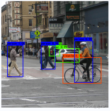
推理结果为