(一)选题背景:
1.生物多样性保护:鸟类是地球上最为丰富和多样的脊椎动物类群之一,对于生态系统的稳定和生物多样性的维持起着重要作用。通过开展鸟类图像分类研究,可以帮助精确地辨别鸟类物种,有助于监测鸟类的分布、数量和迁徙情况,从而更好地实施生物多样性保护和生态环境管理。2.环境监测和生态学研究:鸟类在各种不同的生态系统中都占据着特定的生态角色,其物种组成和数量分布可以反映出环境质量和生态系统变化。通过对鸟类图像进行分类和监测,可以在大尺度上了解不同地区的生态系统状态、环境变化以及人类活动对生态系统的影响。
3.计算机视觉和深度学习研究:鸟类图像分类是计算机视觉领域的经典问题,涉及图像分割、特征提取、对象识别和模式识别等技术。通过开展鸟类图像分类研究,可以推动计算机视觉和深度学习在实际场景中的应用和发展,促进相关算法和模型的优化和改进。
数据集来源:kaggle,网址:https://www.kaggle.com/
(二)机器学习的实现步骤
1.数据集下载


2.导入需要用到的库
 1 import warnings
 2 from sklearn.exceptions import ConvergenceWarning
 3 warnings.filterwarnings("ignore", category=ConvergenceWarning)
 4 warnings.simplefilter(action='ignore', category=FutureWarning)
 5 warnings.simplefilter(action='ignore', category=UserWarning)
 6
 7 import itertools
 8 import numpy as np
 9 import pandas as pd
10 import os
11 import matplotlib.pyplot as plt
12 from sklearn.preprocessing import LabelEncoder
13 from sklearn.model_selection import train_test_split
14 from PIL import Image
15 from sklearn.metrics import classification_report, f1_score , confusion_matrix
16
17
18
19 # Tensorflow库
20 import tensorflow as tf
21 from tensorflow import keras
22 from keras.layers import Dense, Dropout , BatchNormalization
23 from tensorflow.keras.optimizers import Adam
24 from tensorflow.keras import layers,models,Model
25 from keras.preprocessing.image import ImageDataGenerator
26 from tensorflow.keras.layers.experimental import preprocessing
27 from tensorflow.keras.callbacks import Callback, EarlyStopping, ModelCheckpoint, ReduceLROnPlateau
28 from tensorflow.keras import mixed_precision
29 mixed_precision.set_global_policy('mixed_float16')
30
31
32 print(tf.__version__)

3.加载数据
 1 # 定义数据集路径
 2 dataset = {
 3              "train_data" : "./lty/input/bird-species/train",
 4              "valid_data" : "./lty/input/bird-species/valid",
 5              "test_data" : "./lty/input/bird-species/test"
 6           }
 7
 8 all_data = []
 9
10 # 遍历数据集文件夹并读取图片和标签信息
11 for path in dataset.values():
12     data = {"imgpath": [] , "labels": [] }
13     category = os.listdir(path)
14
15     for folder in category:
16         folderpath = os.path.join(path , folder)
17         filelist = os.listdir(folderpath)
18         for file in filelist:
19             fpath = os.path.join(folderpath, file)
20             data["imgpath"].append(fpath)
21             data["labels"].append(folder)
22
23     # 将数据加入列表中
24     all_data.append(data.copy())
25     data.clear()
26
27 # 将列表转化为DataFrame格式
28 train_df = pd.DataFrame(all_data[0] , index=range(len(all_data[0]['imgpath'])))
29 valid_df = pd.DataFrame(all_data[1] , index=range(len(all_data[1]['imgpath'])))
30 test_df = pd.DataFrame(all_data[2] , index=range(len(all_data[2]['imgpath'])))
31
32 # 将标签转化为数字编码
33 lb = LabelEncoder()
34 train_df['encoded_labels'] = lb.fit_transform(train_df['labels'])
35 valid_df['encoded_labels'] = lb.fit_transform(valid_df['labels'])
36 test_df['encoded_labels'] = lb.fit_transform(test_df['labels'])
 1 # 获取训练集中每个类别的图像数量和标签
 2 train  = train_df["labels"].value_counts()
 3 label = train.tolist()
 4 index = train.index.tolist()
 5
 6 # 设置颜色列表
 7 colors = [
 8     "#1f77b4", "#ff7f0e", "#2ca02c", "#d62728", "#9467bd",
 9     "#8c564b", "#e377c2", "#7f7f7f", "#bcbd22", "#17becf",
10     "#aec7e8", "#ffbb78", "#98df8a", "#ff9896", "#c5b0d5",
11     "#c49c94", "#f7b6d2", "#c7c7c7", "#dbdb8d", "#9edae5",
12     "#5254a3", "#6b6ecf", "#bdbdbd", "#8ca252", "#bd9e39",
13     "#ad494a", "#8c6d31", "#6b6ecf", "#e7ba52", "#ce6dbd",
14     "#9c9ede", "#cedb9c", "#de9ed6", "#ad494a", "#d6616b",
15     "#f7f7f7", "#7b4173", "#a55194", "#ce6dbd"
16 ]
17
18 # 绘制水平条形图
19 plt.figure(figsize=(30,30))
20 plt.title("Training data images count per class",fontsize=38)
21 plt.xlabel('Number of images', fontsize=35)
22 plt.ylabel('Classes', fontsize=35)
23 plt.barh(index,label, color=colors)
24 plt.grid(True)
25 plt.show()

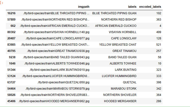
1 # 从训练集中随机选择15个样本
2 train_df.sample(n=15, random_state=1)
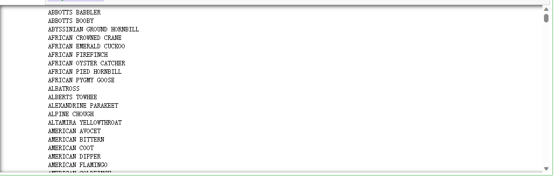
 1 import os
 2
 3 # 设置训练集文件夹路径
 4 path = "C:/Users/z/lty/bird-species/train"
 5
 6 # 获取train训练集文件夹列表
 7 dirs = os.listdir(path)
 8
 9 # 遍历文件夹列表并打印文件名
10 for file in dirs:
11     print(file)
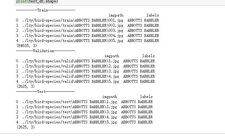
 1 # 打印训练集信息
 2 print("----------Train-------------")
 3 print(train_df[["imgpath", "labels"]].head(5))  # 打印前5行的图像路径和标签
 4 print(train_df.shape)  # 打印训练集的形状,即行数和列数
 5
 6 # 打印验证集信息
 7 print("--------Validation----------")
 8 print(valid_df[["imgpath", "labels"]].head(5))  # 打印前5行的图像路径和标签
 9 print(valid_df.shape)  # 打印验证集的形状,即行数和列数
10
11 # 打印测试集信息
12 print("----------Test--------------")
13 print(test_df[["imgpath", "labels"]].head(5))  # 打印前5行的图像路径和标签
14 print(test_df.shape)  # 打印测试集的形状,即行数和列数
4.展示数据的样本
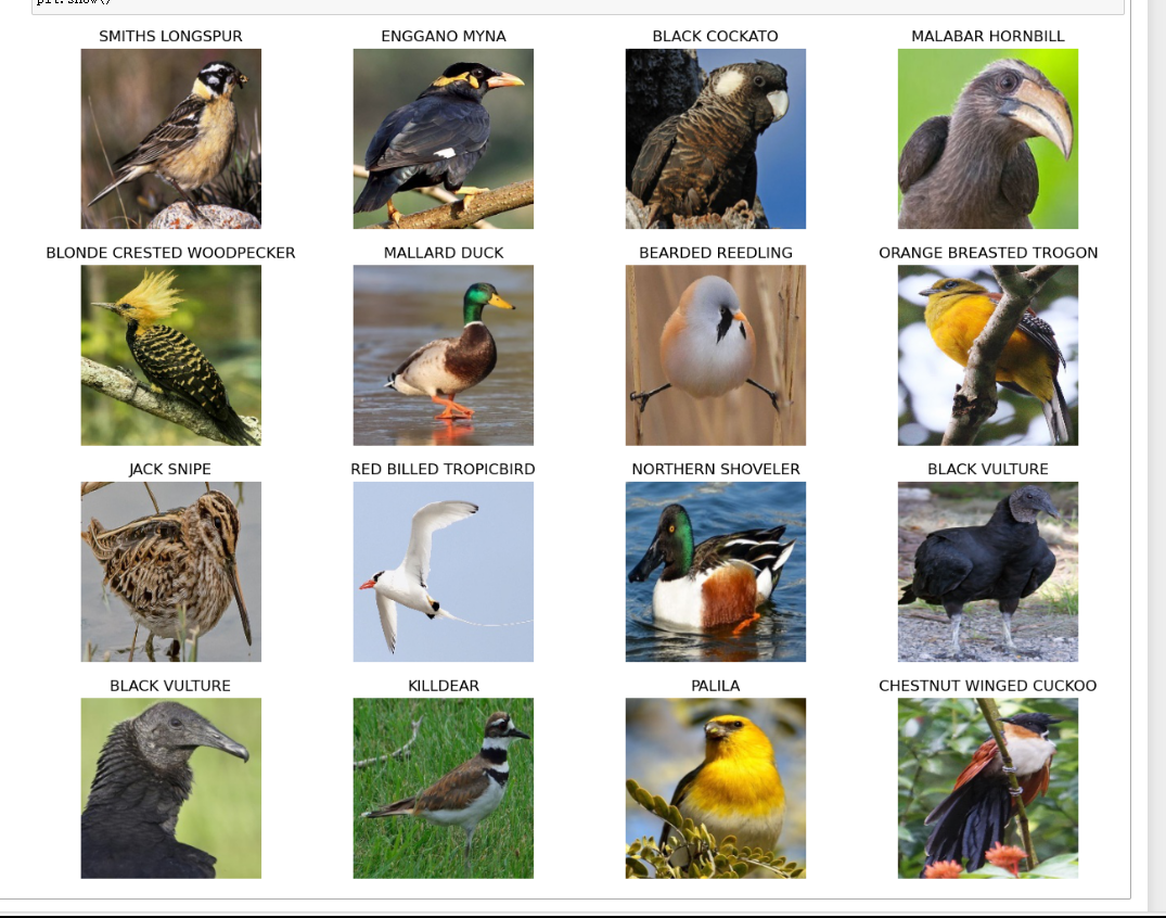
 1 import matplotlib.pyplot as plt
 2 from PIL import Image
 3
 4 # 创建一个大小为15x12的画布
 5 plt.figure(figsize=(15, 12))
 6
 7 # 从验证集中随机选择16个样本,重置索引并逐行处理
 8 for i, row in valid_df.sample(n=16).reset_index().iterrows():
 9     # 在4x4的子图中的第i+1个位置创建一个子图
10     plt.subplot(4, 4, i+1)
11
12     # 获取图像路径
13     image_path = row['imgpath']
14
15     image = Image.open(image_path)
16
17     plt.imshow(image)
18
19     # 设置子图的标题为标签值
20     plt.title(row["labels"])
21
22     plt.axis('off')
23 plt.show()
5.创建数据加载器(Dataloaders)
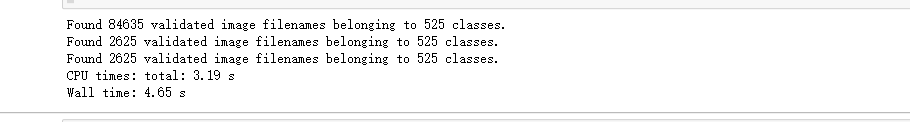
 1 %%time
 2
 3 BATCH_SIZE = 35
 4 IMAGE_SIZE = (224, 224)
 5
 6 # 导入图像数据生成器 ImageDataGenerator
 7 from keras.preprocessing.image import ImageDataGenerator
 8
 9 # 定义数据增强生成器
10 generator = ImageDataGenerator(
11     preprocessing_function=tf.keras.applications.efficientnet.preprocess_input,  # 预处理函数
12     rescale=1./255,  # 将像素值缩放到0-1之间
13     width_shift_range=0.2,  # 水平和垂直方向上的随机平移范围
14     height_shift_range=0.2,
15     zoom_range=0.2  # 随机缩放图像的范围
16 )
17
18 # 将训练集数据分批生成并进行数据增强
19 train_images = generator.flow_from_dataframe(
20     dataframe=train_df,  # 使用train_df作为数据源
21     x_col='imgpath',  # 图像路径的列名
22     y_col='labels',  # 标签的列名
23     target_size=IMAGE_SIZE,  # 图像的目标大小
24     color_mode='rgb',  # 图像的颜色通道模式
25     class_mode='categorical',  # 分类模式,输出是一个one-hot编码的向量
26     batch_size=BATCH_SIZE,  # 批次大小
27     shuffle=True,  # 是否打乱数据顺序
28     seed=42  # 随机种子
29 )
30
31 # 将验证集数据分批生成
32 val_images = generator.flow_from_dataframe(
33     dataframe=valid_df,  # 使用valid_df作为数据源
34     x_col='imgpath',
35     y_col='labels',
36     target_size=IMAGE_SIZE,
37     color_mode='rgb',
38     class_mode='categorical',
39     batch_size=BATCH_SIZE,
40     shuffle=False
41 )
42
43 # 将测试集数据分批生成
44 test_images = generator.flow_from_dataframe(
45     dataframe=test_df,  # 使用test_df作为数据源
46     x_col='imgpath',
47     y_col='labels',
48     target_size=IMAGE_SIZE,
49     color_mode='rgb',
50     class_mode='categorical',
51     batch_size=BATCH_SIZE,
52     shuffle=False
53 )
1 train_images[0][0].shape

1 img= train_images[0]
2 print(img)
1 type(train_images)

1 img = train_images[0]
2 print(img[0].shape)
3 print(img[1].shape)

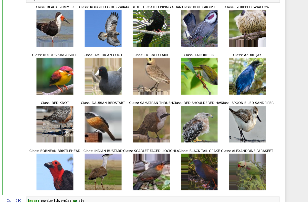
 1 labels = [k for k in train_images.class_indices]
 2 sample_images = train_images.__next__()
 3
 4 images = sample_generate[0]
 5 titles = sample_generate[1]
 6 plt.figure(figsize = (15 , 15))
 7
 8 for i in range(20):
 9     plt.subplot(5 ,  5 , i+1)
10     plt.subplots_adjust(hspace = 0.3 , wspace = 0.3)#调整子图之间的空白区域
11     plt.imshow(images[i])
12     plt.title(f'Class: {labels[np.argmax(titles[i],axis=0)]}')
13     plt.axis("off")
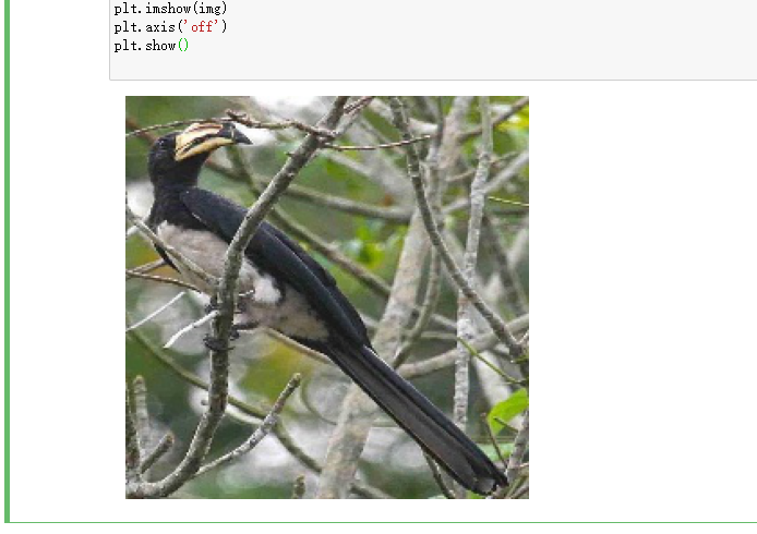
1 import matplotlib.pyplot as plt
2 from skimage import io
3
4 img_url = "./lty/bird-species/train/AFRICAN PIED HORNBILL/007.jpg"#指定要读取和显示的图像文件路径
5 img = io.imread(img_url)#imread函数以数组形式读取指定路径下的图像文件
6
7 plt.imshow(img)
8 plt.axis('off')
9 plt.show()
 1 # 加载预训练模型
 2 pretrained_model = tf.keras.applications.EfficientNetB5(
 3     input_shape=(224, 224, 3),
 4     include_top=False, # 不加载或重新初始化顶层(输出层)的参数
 5     weights='imagenet',
 6     pooling='max'
 7 )
 8
 9 # 冻结预训练神经网络的层
10 for i, layer in enumerate(pretrained_model.layers):
11     pretrained_model.layers[i].trainable = False

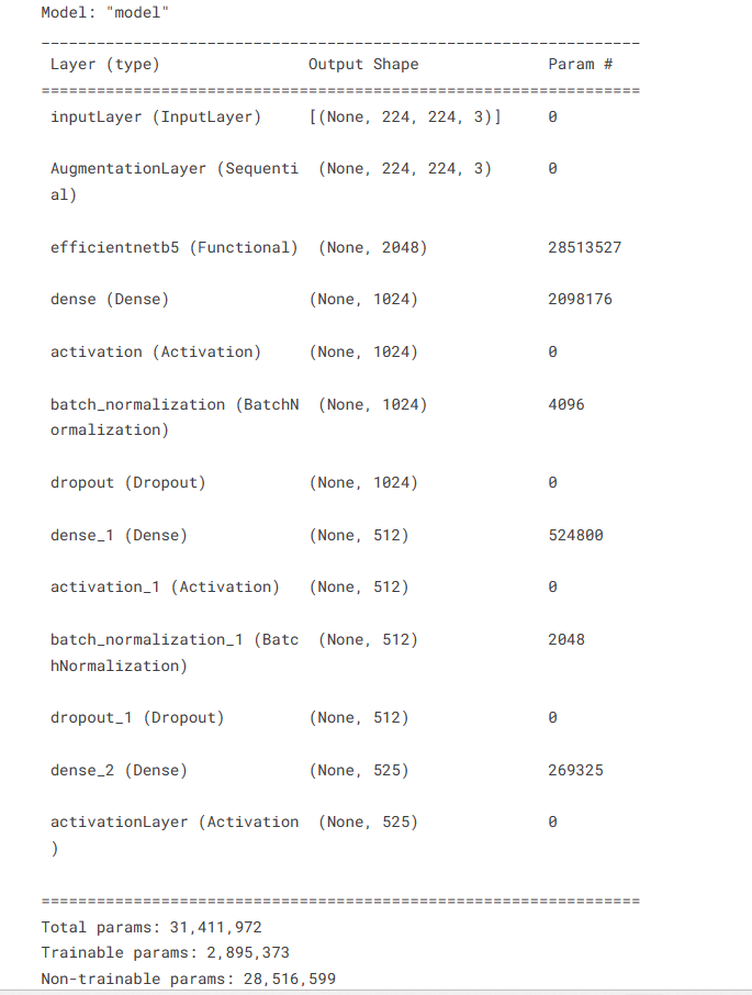
 1 # 获取类别数
 2 num_classes = len(set(train_images.classes))
 3
 4 # 对数据进行增强
 5 augment = tf.keras.Sequential([
 6   layers.experimental.preprocessing.RandomFlip("horizontal"),
 7   layers.experimental.preprocessing.RandomRotation(0.15),
 8   layers.experimental.preprocessing.RandomZoom(0.12),
 9   layers.experimental.preprocessing.RandomContrast(0.12),
10 ], name='AugmentationLayer')
11
12 # 输入层
13 inputs = layers.Input(shape=(224, 224, 3), name='inputLayer')
14 x = augment(inputs)  # 应用数据增强
15 pretrain_out = pretrained_model(x, training=False)
16
17 # 添加全连接层和激活函数
18 x = layers.Dense(1024)(pretrain_out)
19 x = layers.Activation(activation="relu")(x)
20 x = BatchNormalization()(x)
21 x = layers.Dropout(0.45)(x)
22 x = layers.Dense(512)(x)
23 x = layers.Activation(activation="relu")(x)
24 x = BatchNormalization()(x)
25 x = layers.Dropout(0.3)(x)
26 x = layers.Dense(num_classes)(x)
27 outputs = layers.Activation(activation="softmax", dtype=tf.float32, name='activationLayer')(x)
28
29 # 创建模型
30 model = Model(inputs=inputs, outputs=outputs)
31
32 # 编译模型
33 model.compile(
34     optimizer=Adam(0.0005),
35     loss='categorical_crossentropy',
36     metrics=['accuracy']
37 )
38
39 # 打印模型结构摘要
40 print(model.summary())
6.预训练模型
在 transfer learning 中,我们可以选择保持预训练模型的一部分或全部参数不变(称为冻结),只对最后几层或某些层进行微调,以适应新任务的特定要求。这样做的原因是预训练模型已经学习到了通用的特征,我们可以认为这些特征对于新任务也是有用的。通过仅微调少量参数,我们可以在较小的数据集上快速训练出具有良好性能的模型。
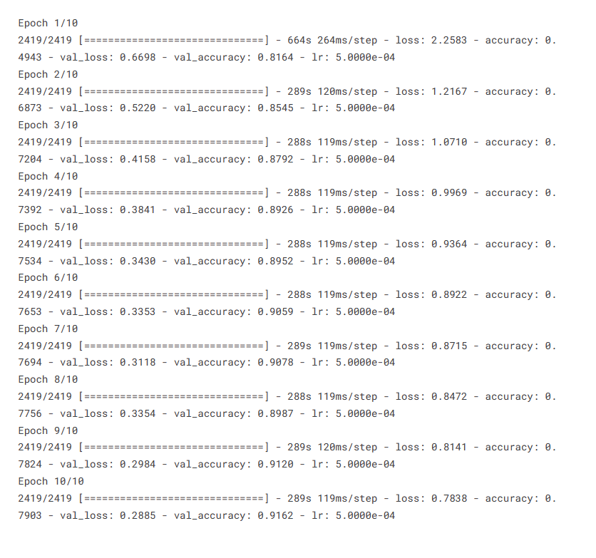
 1 # 训练模型
 2 history = model.fit(
 3     train_images,
 4     steps_per_epoch=len(train_images),
 5     validation_data=val_images,
 6     validation_steps=len(val_images),
 7     epochs=10,
 8     callbacks=[
 9         # 提前停止回调,如果验证集损失在连续3个epoch中没有改善,则提前停止训练
10         EarlyStopping(monitor="val_loss", patience=3, restore_best_weights=True),
11         # 学习率调整,在验证集损失没有改善时降低学习率
12         ReduceLROnPlateau(monitor='val_loss', factor=0.2, patience=2, mode='min')
13     ]
14 )
15
16 # 保存模型权重
17 model.save_weights('./lty/input/bird-species/my_checkpoint')
7.模型的性能
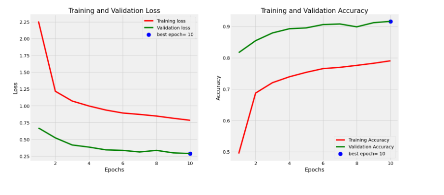
 1 # 定义所需变量
 2 tr_acc = history.history['accuracy']  # 训练准确率
 3 tr_loss = history.history['loss']  # 训练损失
 4 val_acc = history.history['val_accuracy']  # 验证准确率
 5 val_loss = history.history['val_loss']  # 验证损失
 6 index_loss = np.argmin(val_loss)  # 最小验证损失的索引
 7 val_lowest = val_loss[index_loss]  # 最小验证损失
 8 index_acc = np.argmax(val_acc)  # 最大验证准确率的索引
 9 acc_highest = val_acc[index_acc]  # 最大验证准确率
10 Epochs = [i+1 for i in range(len(tr_acc))]  # 训练轮数
11 loss_label = f'best epoch= {str(index_loss + 1)}'  # 最小验证损失的标签
12 acc_label = f'best epoch= {str(index_acc + 1)}'  # 最大验证准确率的标签
13
14 # 绘制训练历史图表
15 plt.figure(figsize=(20, 8))
16 plt.style.use('fivethirtyeight')
17
18 plt.subplot(1, 2, 1)
19 plt.plot(Epochs, tr_loss, 'r', label='Training loss')  # 绘制训练损失曲线
20 plt.plot(Epochs, val_loss, 'g', label='Validation loss')  # 绘制验证损失曲线
21 plt.scatter(index_loss + 1, val_lowest, s=150, c='blue', label=loss_label)  # 标记最小验证损失点
22 plt.title('Training and Validation Loss')
23 plt.xlabel('Epochs')
24 plt.ylabel('Loss')
25 plt.legend()
26
27 plt.subplot(1, 2, 2)
28 plt.plot(Epochs, tr_acc, 'r', label='Training Accuracy')  # 绘制训练准确率曲线
29 plt.plot(Epochs, val_acc, 'g', label='Validation Accuracy')  # 绘制验证准确率曲线
30 plt.scatter(index_acc + 1, acc_highest, s=150, c='blue', label=acc_label)  # 标记最大验证准确率点
31 plt.title('Training and Validation Accuracy')
32 plt.xlabel('Epochs')
33 plt.ylabel('Accuracy')
34 plt.legend()
35
36 plt.tight_layout()
37 plt.show()
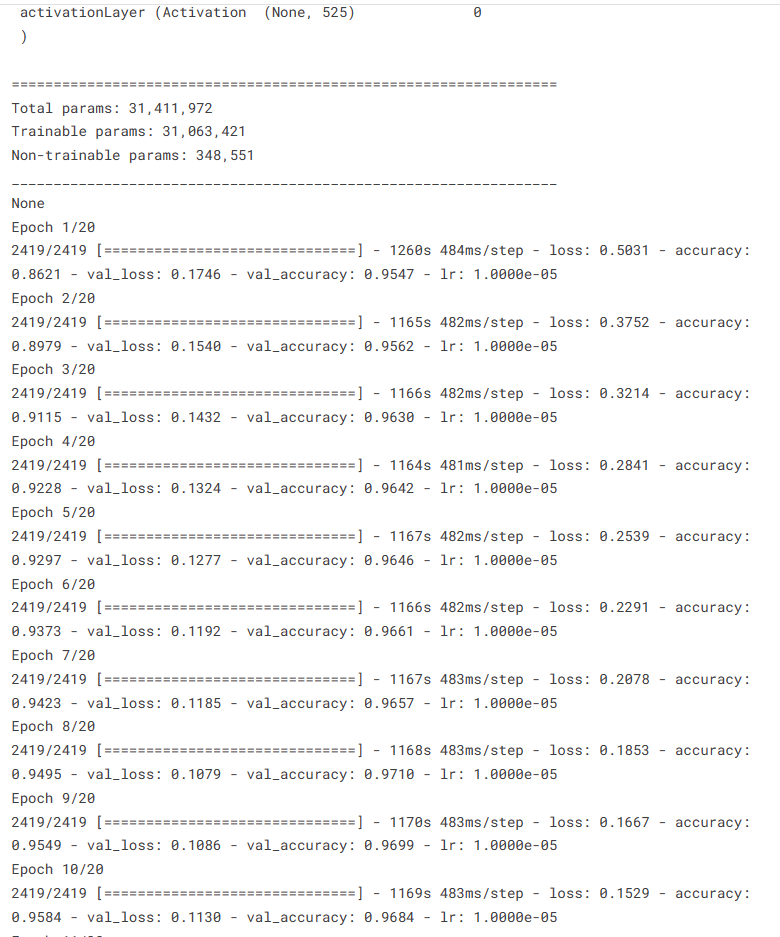
8.对预训练模型进行微调
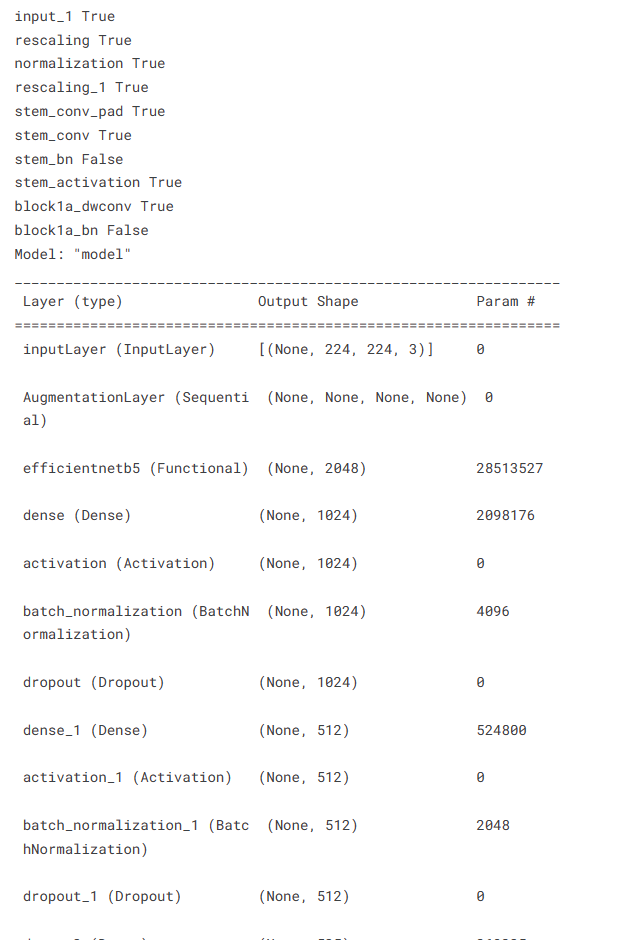
 1 pretrained_model.trainable = True
 2 for layer in pretrained_model.layers:
 3     if isinstance(layer, layers.BatchNormalization): # 将 BatchNorm 层设置为不可训练,冻结 BatchNorm 层的参数
 4         layer.trainable = False
 5
 6 # 查看深度学习模型的前 10 层
 7 for l in pretrained_model.layers[:10]:
 8     print(l.name, l.trainable)
 9
10 model.compile(
11     optimizer=Adam(0.00001), # 使用小学习率进行微调
12     loss='categorical_crossentropy',
13     metrics=['accuracy']
14 )
15 # model.load_weights('./lty/bird-species/my_checkpoint')
16 print(model.summary())
17 history = model.fit(
18     train_images,
19     steps_per_epoch=len(train_images),
20     validation_data=val_images,
21     validation_steps=len(val_images),
22     epochs=20,
23     callbacks=[
24         EarlyStopping(monitor = "val_loss", # 观察验证集的损失指标
25                                patience = 5,
26                                restore_best_weights = True), # if val loss decreases for 5 epochs in a row, stop training,
27         ReduceLROnPlateau(monitor='val_loss', factor=0.2, patience=2, mode='min')
28     ]
29 )
30 model.save_weights('./lty/bird-species/my_checkpoint')
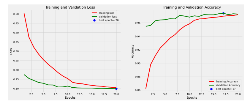
 1 # 定义所需的变量
 2 tr_acc = history.history['accuracy']
 3 tr_loss = history.history['loss']
 4 val_acc = history.history['val_accuracy']
 5 val_loss = history.history['val_loss']
 6 index_loss = np.argmin(val_loss)
 7 val_lowest = val_loss[index_loss]
 8 index_acc = np.argmax(val_acc)
 9 acc_highest = val_acc[index_acc]
10 Epochs = [i+1 for i in range(len(tr_acc))]
11 loss_label = f'best epoch= {str(index_loss + 1)}'
12 acc_label = f'best epoch= {str(index_acc + 1)}'
13
14 # 绘制训练历史
15 plt.figure(figsize= (20, 8))
16 plt.style.use('fivethirtyeight')
17
18 plt.subplot(1, 2, 1)
19 plt.plot(Epochs, tr_loss, 'r', label= 'Training loss')
20 plt.plot(Epochs, val_loss, 'g', label= 'Validation loss')
21 plt.scatter(index_loss + 1, val_lowest, s= 150, c= 'blue', label= loss_label)
22 plt.title('Training and Validation Loss')
23 plt.xlabel('Epochs')
24 plt.ylabel('Loss')
25 plt.legend()
26
27 plt.subplot(1, 2, 2)
28 plt.plot(Epochs, tr_acc, 'r', label= 'Training Accuracy')
29 plt.plot(Epochs, val_acc, 'g', label= 'Validation Accuracy')
30 plt.scatter(index_acc + 1 , acc_highest, s= 150, c= 'blue', label= acc_label)
31 plt.title('Training and Validation Accuracy')
32 plt.xlabel('Epochs')
33 plt.ylabel('Accuracy')
34 plt.legend()
35
36 plt.tight_layout
37 plt.show()
9.评估模型在给定数据集上的性能
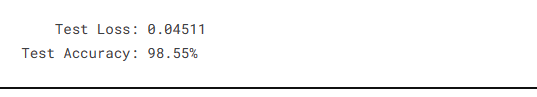
1 results = model.evaluate(test_images, verbose=0)
2  # 对测试集进行评估,返回测试损失和测试准确率
3
4 print("    Test Loss: {:.5f}".format(results[0]))
5  # 打印测试损失,保留小数点后5位
6 print("Test Accuracy: {:.2f}%".format(results[1] * 100))
7 # 打印测试准确率,乘以100后保留两位小数
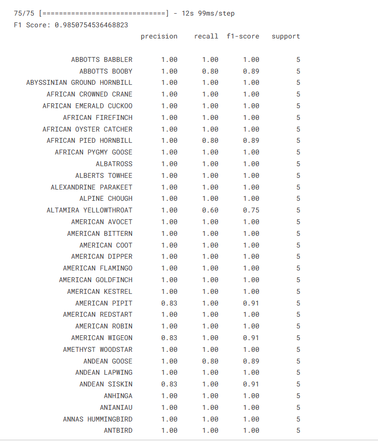
1 y_true = test_images.classes  # 获取测试集样本的真实标签
2 y_pred = np.argmax(model.predict(test_images), axis=1)
3 # 获取模型对测试集样本的预测标签
4
5 # 计算并打印F1 Score和分类报告
6 f1 = f1_score(y_true, y_pred, average='macro')  # 计算F1 Score
7 print("F1 Score:", f1)
8 print(classification_report(y_true, y_pred, target_names=test_images.class_indices.keys()))  # 打印分类报告
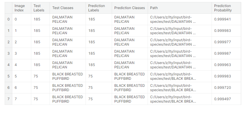
10.获取预测结果
 1 # 创建一个字典,将类别索引和对应的类别名称进行关联
 2 classes = dict(zip(test_images.class_indices.values(), test_images.class_indices.keys()))
 3
 4 # 创建一个DataFrame来存储预测结果
 5 Predictions = pd.DataFrame({
 6     "Image Index": list(range(len(test_images.labels))),  # 图像索引
 7     "Test Labels": test_images.labels,  # 真实标签
 8     "Test Classes": [classes[i] for i in test_images.labels],  # 真实类别
 9     "Prediction Labels": y_pred,  # 预测标签
10     "Prediction Classes": [classes[i] for i in y_pred],  # 预测类别
11     "Path": test_images.filenames,  # 图像路径
12     "Prediction Probability": [x for x in np.asarray(tf.reduce_max(model.predict(test_images), axis=1))]  # 预测概率
13 })
14
15 Predictions.head(8)  # 输出前8行预测结果

11.在测试数据集上预测错误且置信度最高的样本
 1 plt.figure(figsize=(20, 20))
 2 # 选择分类错误的预测结果中概率最高的20个样本
 3 subset = Predictions[Predictions["Test Labels"] != Predictions["Prediction Labels"]].sort_values("Prediction Probability").tail(20).reset_index()
 4
 5 for i, row in subset.iterrows():
 6     plt.subplot(5, 4, i+1)
 7     image_path = row['Path']
 8     image = Image.open(image_path)
 9     # 显示图像
10     plt.imshow(image)
11     # 设置图像标题,包括真实类别和预测类别
12     plt.title(f'TRUE: {row["Test Classes"]} | PRED: {row["Prediction Classes"]}', fontsize=8)
13     plt.axis('off')
14
15 plt.show()

13. 评估分类模型性能
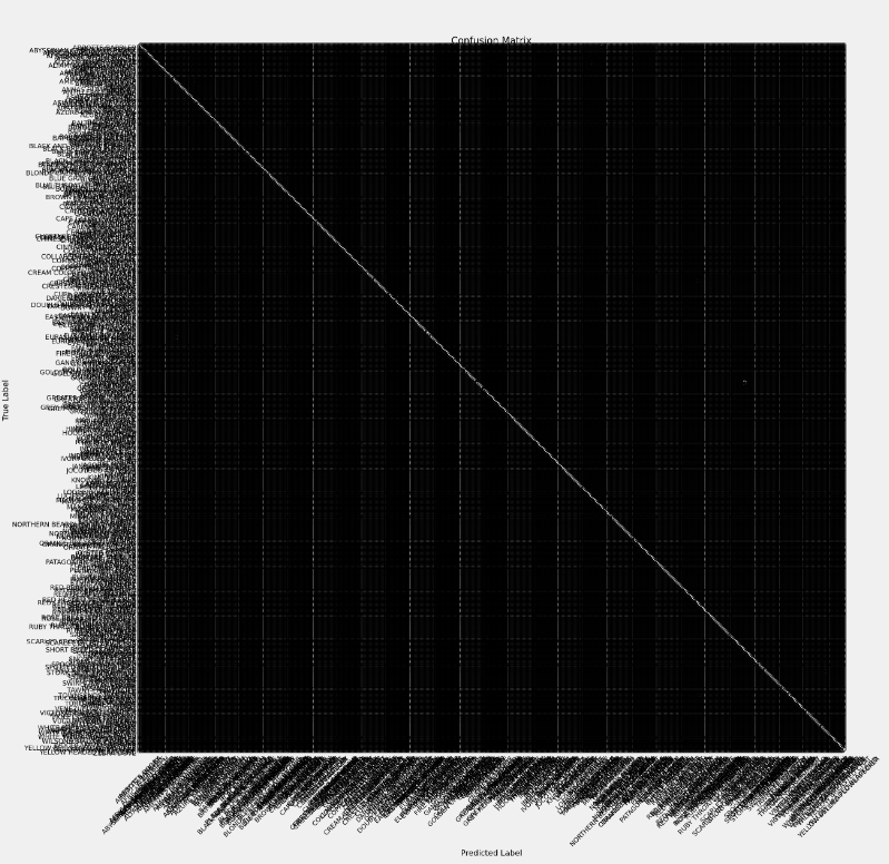
混淆矩阵(Confusion Matrix)和分类报告(Classification Report)
 1 import numpy as np
 2 from sklearn.metrics import confusion_matrix
 3 import itertools
 4 import matplotlib.pyplot as plt
 5
 6 # 使用模型对测试图片进行预测
 7 preds = model.predict_generator(test_images)
 8 # 找到每个预测结果中概率最高的类别作为预测标签
 9 y_pred = np.argmax(preds, axis=1)
10
11 # 获取测试图片的真实标签和对应的类别字典
12 g_dict = test_images.class_indices
13 # 创建一个包含所有类别名称的列表
14 classes = list(g_dict.keys())
15
16 # 计算混淆矩阵
17 cm = confusion_matrix(test_images.classes, y_pred)
18
19 plt.figure(figsize=(30, 30))
20 plt.imshow(cm, interpolation='nearest', cmap=plt.cm.Blues)
21 plt.title('Confusion Matrix')
22 plt.colorbar()
23
24 tick_marks = np.arange(len(classes))
25 plt.xticks(tick_marks, classes, rotation=45)
26 plt.yticks(tick_marks, classes)
27
28 thresh = cm.max() / 2.
29 for i, j in itertools.product(range(cm.shape[0]), range(cm.shape[1])):
30     plt.text(j, i, cm[i, j], horizontalalignment='center', color='white' if cm[i, j] > thresh else 'black')
31
32 plt.tight_layout()
33 plt.ylabel('True Label')
34 plt.xlabel('Predicted Label')
35
36 plt.show()
使用matplotlib库绘制了一个大小为30x30的图像窗口,显示了混淆矩阵的热力图。热力图的颜色越深,表示预测结果越准确。图像中的数字表示每个混淆矩阵单元格中的样本数量。图像上方的标题为"Confusion Matrix",颜色条表示每个颜色对应的样本数量范围。x轴标签为预测标签,y轴标签为真实标签。
总代码
  1 import warnings
  2 from sklearn.exceptions import ConvergenceWarning
  3 warnings.filterwarnings("ignore", category=ConvergenceWarning)
  4 warnings.simplefilter(action='ignore', category=FutureWarning)
  5 warnings.simplefilter(action='ignore', category=UserWarning)
  6
  7 # 导入必要的库
  8 import itertools
  9 import numpy as np
 10 import pandas as pd
 11 import os
 12 import matplotlib.pyplot as plt
 13 from sklearn.preprocessing import LabelEncoder
 14 from sklearn.model_selection import train_test_split
 15 from PIL import Image
 16 from sklearn.metrics import classification_report, f1_score , confusion_matrix
 17
 18 # 导入TensorFlow库
 19 import tensorflow as tf
 20 from tensorflow import keras
 21 from keras.layers import Dense, Dropout , BatchNormalization
 22 from tensorflow.keras.optimizers import Adam
 23 from tensorflow.keras import layers,models,Model
 24 from keras.preprocessing.image import ImageDataGenerator
 25 from tensorflow.keras.layers.experimental import preprocessing
 26 from tensorflow.keras.callbacks import Callback, EarlyStopping, ModelCheckpoint, ReduceLROnPlateau
 27 from tensorflow.keras import mixed_precision
 28 mixed_precision.set_global_policy('mixed_float16')
 29
 30 # 输出TensorFlow版本
 31 print(tf.__version__)
 32
 33
 34 # 定义数据集路径
 35 dataset = {
 36              "train_data" : "./lty/input/bird-species/train",
 37              "valid_data" : "./lty/input/bird-species/valid",
 38              "test_data" : "./lty/input/bird-species/test"
 39           }
 40
 41 all_data = []
 42
 43 # 遍历数据集文件夹并读取图片和标签信息
 44 for path in dataset.values():
 45     data = {"imgpath": [] , "labels": [] }
 46     category = os.listdir(path)
 47
 48     for folder in category:
 49         folderpath = os.path.join(path , folder)
 50         filelist = os.listdir(folderpath)
 51         for file in filelist:
 52             fpath = os.path.join(folderpath, file)
 53             data["imgpath"].append(fpath)
 54             data["labels"].append(folder)
 55
 56     # 将数据加入列表中
 57     all_data.append(data.copy())
 58     data.clear()
 59
 60 # 将列表转化为DataFrame格式
 61 train_df = pd.DataFrame(all_data[0] , index=range(len(all_data[0]['imgpath'])))
 62 valid_df = pd.DataFrame(all_data[1] , index=range(len(all_data[1]['imgpath'])))
 63 test_df = pd.DataFrame(all_data[2] , index=range(len(all_data[2]['imgpath'])))
 64
 65 # 将标签转化为数字编码
 66 lb = LabelEncoder()
 67 train_df['encoded_labels'] = lb.fit_transform(train_df['labels'])
 68 valid_df['encoded_labels'] = lb.fit_transform(valid_df['labels'])
 69 test_df['encoded_labels'] = lb.fit_transform(test_df['labels'])
 70
 71 # 获取训练集中每个类别的图像数量和标签
 72 train  = train_df["labels"].value_counts()
 73 label = train.tolist()
 74 index = train.index.tolist()
 75
 76 # 设置颜色列表
 77 colors = [
 78     "#1f77b4", "#ff7f0e", "#2ca02c", "#d62728", "#9467bd",
 79     "#8c564b", "#e377c2", "#7f7f7f", "#bcbd22", "#17becf",
 80     "#aec7e8", "#ffbb78", "#98df8a", "#ff9896", "#c5b0d5",
 81     "#c49c94", "#f7b6d2", "#c7c7c7", "#dbdb8d", "#9edae5",
 82     "#5254a3", "#6b6ecf", "#bdbdbd", "#8ca252", "#bd9e39",
 83     "#ad494a", "#8c6d31", "#6b6ecf", "#e7ba52", "#ce6dbd",
 84     "#9c9ede", "#cedb9c", "#de9ed6", "#ad494a", "#d6616b",
 85     "#f7f7f7", "#7b4173", "#a55194", "#ce6dbd"
 86 ]
 87
 88 # 绘制水平条形图
 89 plt.figure(figsize=(30,30))
 90 plt.title("Training data images count per class",fontsize=38)
 91 plt.xlabel('Number of images', fontsize=35)
 92 plt.ylabel('Classes', fontsize=35)
 93 plt.barh(index,label, color=colors)
 94 plt.grid(True)
 95 plt.show()
 96
 97
 98 # 从训练集中随机选择15个样本
 99 train_df.sample(n=15, random_state=1)
100
101
102 import os
103
104 # 设置训练集文件夹路径
105 path = "C:/Users/z/lty/bird-species/train"
106
107 # 获取train训练集文件夹列表
108 dirs = os.listdir(path)
109
110 # 遍历文件夹列表并打印文件名
111 for file in dirs:
112     print(file)
113
114
115 # 打印训练集信息
116 print("----------Train-------------")
117 print(train_df[["imgpath", "labels"]].head(5))  # 打印前5行的图像路径和标签
118 print(train_df.shape)  # 打印训练集的形状,即行数和列数
119
120 # 打印验证集信息
121 print("--------Validation----------")
122 print(valid_df[["imgpath", "labels"]].head(5))  # 打印前5行的图像路径和标签
123 print(valid_df.shape)  # 打印验证集的形状,即行数和列数
124
125 # 打印测试集信息
126 print("----------Test--------------")
127 print(test_df[["imgpath", "labels"]].head(5))  # 打印前5行的图像路径和标签
128 print(test_df.shape)  # 打印测试集的形状,即行数和列数
129
130 import matplotlib.pyplot as plt
131 from PIL import Image
132
133 # 创建一个大小为15x12的画布
134 plt.figure(figsize=(15, 12))
135
136 # 从验证集中随机选择16个样本,重置索引并逐行处理
137 for i, row in valid_df.sample(n=16).reset_index().iterrows():
138     # 在4x4的子图中的第i+1个位置创建一个子图
139     plt.subplot(4, 4, i+1)
140
141     # 获取图像路径
142     image_path = row['imgpath']
143
144     image = Image.open(image_path)
145
146     plt.imshow(image)
147
148     # 设置子图的标题为标签值
149     plt.title(row["labels"])
150
151     plt.axis('off')
152 plt.show()
153
154
155 %%time
156
157 BATCH_SIZE = 35
158 IMAGE_SIZE = (224, 224)
159
160 # 导入图像数据生成器 ImageDataGenerator
161 from keras.preprocessing.image import ImageDataGenerator
162
163 # 定义数据增强生成器
164 generator = ImageDataGenerator(
165     preprocessing_function=tf.keras.applications.efficientnet.preprocess_input,  # 预处理函数
166     rescale=1./255,  # 将像素值缩放到0-1之间
167     width_shift_range=0.2,  # 水平和垂直方向上的随机平移范围
168     height_shift_range=0.2,
169     zoom_range=0.2  # 随机缩放图像的范围
170 )
171
172 # 将训练集数据分批生成并进行数据增强
173 train_images = generator.flow_from_dataframe(
174     dataframe=train_df,  # 使用train_df作为数据源
175     x_col='imgpath',  # 图像路径的列名
176     y_col='labels',  # 标签的列名
177     target_size=IMAGE_SIZE,  # 图像的目标大小
178     color_mode='rgb',  # 图像的颜色通道模式
179     class_mode='categorical',  # 分类模式,输出是一个one-hot编码的向量
180     batch_size=BATCH_SIZE,  # 批次大小
181     shuffle=True,  # 是否打乱数据顺序
182     seed=42  # 随机种子
183 )
184
185 # 将验证集数据分批生成
186 val_images = generator.flow_from_dataframe(
187     dataframe=valid_df,  # 使用valid_df作为数据源
188     x_col='imgpath',
189     y_col='labels',
190     target_size=IMAGE_SIZE,
191     color_mode='rgb',
192     class_mode='categorical',
193     batch_size=BATCH_SIZE,
194     shuffle=False
195 )
196
197 # 将测试集数据分批生成
198 test_images = generator.flow_from_dataframe(
199     dataframe=test_df,  # 使用test_df作为数据源
200     x_col='imgpath',
201     y_col='labels',
202     target_size=IMAGE_SIZE,
203     color_mode='rgb',
204     class_mode='categorical',
205     batch_size=BATCH_SIZE,
206     shuffle=False
207 )
208
209 train_images[0][0].shape
210
211 img= train_images[0]
212 print(img)
213
214 type(train_images)
215
216 img = train_images[0]
217 print(img[0].shape)
218 print(img[1].shape)
219
220 labels = [k for k in train_images.class_indices]
221 sample_images = train_images.__next__()
222
223 images = sample_images[0]
224 titles = sample_images[1]
225 plt.figure(figsize = (15 , 15))
226
227 for i in range(20):
228     plt.subplot(5 ,  5 , i+1)
229     plt.subplots_adjust(hspace = 0.3 , wspace = 0.3)#调整子图之间的空白区域
230     plt.imshow(images[i])
231     plt.title(f'Class: {labels[np.argmax(titles[i],axis=0)]}')
232     plt.axis("off")
233
234 import matplotlib.pyplot as plt
235 from skimage import io
236
237 img_url = "./lty/input/bird-species/train/AFRICAN PIED HORNBILL/007.jpg"#指定要读取和显示的图像文件路径
238 img = io.imread(img_url)#imread函数以数组形式读取指定路径下的图像文件
239
240 plt.imshow(img)
241 plt.axis('off')
242 plt.show()
243
244
245 # 加载预训练模型
246 pretrained_model = tf.keras.applications.EfficientNetB5(
247     input_shape=(224, 224, 3),
248     include_top=False, # 不加载或重新初始化顶层(输出层)的参数
249     weights='imagenet',
250     pooling='max'
251 )
252
253
254 for i, layer in enumerate(pretrained_model.layers):
255     pretrained_model.layers[i].trainable = False
256
257
258 # 获取类别数
259 num_classes = len(set(train_images.classes))
260
261 # 对数据进行增强
262 augment = tf.keras.Sequential([
263   layers.experimental.preprocessing.RandomFlip("horizontal"),
264   layers.experimental.preprocessing.RandomRotation(0.15),
265   layers.experimental.preprocessing.RandomZoom(0.12),
266   layers.experimental.preprocessing.RandomContrast(0.12),
267 ], name='AugmentationLayer')
268
269 # 输入层
270 inputs = layers.Input(shape=(224, 224, 3), name='inputLayer')
271 x = augment(inputs)  # 应用数据增强
272 pretrain_out = pretrained_model(x, training=False)
273
274 # 添加全连接层和激活函数
275 x = layers.Dense(1024)(pretrain_out)
276 x = layers.Activation(activation="relu")(x)
277 x = BatchNormalization()(x)
278 x = layers.Dropout(0.45)(x)
279 x = layers.Dense(512)(x)
280 x = layers.Activation(activation="relu")(x)
281 x = BatchNormalization()(x)
282 x = layers.Dropout(0.3)(x)
283 x = layers.Dense(num_classes)(x)
284 outputs = layers.Activation(activation="softmax", dtype=tf.float32, name='activationLayer')(x)
285
286 # 创建模型
287 model = Model(inputs=inputs, outputs=outputs)
288
289 # 编译模型
290 model.compile(
291     optimizer=Adam(0.0005),
292     loss='categorical_crossentropy',
293     metrics=['accuracy']
294 )
295
296 # 打印模型结构摘要
297 print(model.summary())
298
299
300 # 训练模型
301 history = model.fit(
302     train_images,
303     steps_per_epoch=len(train_images),
304     validation_data=val_images,
305     validation_steps=len(val_images),
306     epochs=10,
307     callbacks=[
308         # 提前停止回调,如果验证集损失在连续3个epoch中没有改善,则提前停止训练
309         EarlyStopping(monitor="val_loss", patience=3, restore_best_weights=True),
310         # 学习率调整,在验证集损失没有改善时降低学习率
311         ReduceLROnPlateau(monitor='val_loss', factor=0.2, patience=2, mode='min')
312     ]
313 )
314
315 # 保存模型权重
316 model.save_weights('./lty/input/bird-species/my_checkpoint')
317
318
319 # 定义所需变量
320 tr_acc = history.history['accuracy']  # 训练准确率
321 tr_loss = history.history['loss']  # 训练损失
322 val_acc = history.history['val_accuracy']  # 验证准确率
323 val_loss = history.history['val_loss']  # 验证损失
324 index_loss = np.argmin(val_loss)  # 最小验证损失的索引
325 val_lowest = val_loss[index_loss]  # 最小验证损失
326 index_acc = np.argmax(val_acc)  # 最大验证准确率的索引
327 acc_highest = val_acc[index_acc]  # 最大验证准确率
328 Epochs = [i+1 for i in range(len(tr_acc))]  # 训练轮数
329 loss_label = f'best epoch= {str(index_loss + 1)}'  # 最小验证损失的标签
330 acc_label = f'best epoch= {str(index_acc + 1)}'  # 最大验证准确率的标签
331
332 # 绘制训练历史图表
333 plt.figure(figsize=(20, 8))
334 plt.style.use('fivethirtyeight')
335
336 plt.subplot(1, 2, 1)
337 plt.plot(Epochs, tr_loss, 'r', label='Training loss')  # 绘制训练损失曲线
338 plt.plot(Epochs, val_loss, 'g', label='Validation loss')  # 绘制验证损失曲线
339 plt.scatter(index_loss + 1, val_lowest, s=150, c='blue', label=loss_label)  # 标记最小验证损失点
340 plt.title('Training and Validation Loss')
341 plt.xlabel('Epochs')
342 plt.ylabel('Loss')
343 plt.legend()
344
345 plt.subplot(1, 2, 2)
346 plt.plot(Epochs, tr_acc, 'r', label='Training Accuracy')  # 绘制训练准确率曲线
347 plt.plot(Epochs, val_acc, 'g', label='Validation Accuracy')  # 绘制验证准确率曲线
348 plt.scatter(index_acc + 1, acc_highest, s=150, c='blue', label=acc_label)  # 标记最大验证准确率点
349 plt.title('Training and Validation Accuracy')
350 plt.xlabel('Epochs')
351 plt.ylabel('Accuracy')
352 plt.legend()
353
354 plt.tight_layout()
355 plt.show()
356
357
358 results = model.evaluate(test_images, verbose=0)
359 # 对测试集进行评估,返回测试损失和测试准确率
360
361 print("    Test Loss: {:.5f}".format(results[0]))
362 # 打印测试损失,保留小数点后5位
363 print("Test Accuracy: {:.2f}%".format(results[1] * 100))
364 # 打印测试准确率,乘以100后保留两位小数
365
366 y_true = test_images.classes  # 获取测试集样本的真实标签
367 y_pred = np.argmax(model.predict(test_images), axis=1)
368 # 获取模型对测试集样本的预测标签
369
370 # 计算并打印F1 Score和分类报告
371 f1 = f1_score(y_true, y_pred, average='macro')  # 计算F1 Score
372 print("F1 Score:", f1)
373 print(classification_report(y_true, y_pred, target_names=test_images.class_indices.keys()))  # 打印分类报告
374
375
376 # 创建一个字典,将类别索引和对应的类别名称进行关联
377 classes = dict(zip(test_images.class_indices.values(), test_images.class_indices.keys()))
378
379 # 创建一个DataFrame来存储预测结果
380 Predictions = pd.DataFrame({
381     "Image Index": list(range(len(test_images.labels))),  # 图像索引
382     "Test Labels": test_images.labels,  # 真实标签
383     "Test Classes": [classes[i] for i in test_images.labels],  # 真实类别
384     "Prediction Labels": y_pred,  # 预测标签
385     "Prediction Classes": [classes[i] for i in y_pred],  # 预测类别
386     "Path": test_images.filenames,  # 图像路径
387     "Prediction Probability": [x for x in np.asarray(tf.reduce_max(model.predict(test_images), axis=1))]  # 预测概率
388 })
389
390 Predictions.head(8)  # 输出前8行预测结果
391
392
393 plt.figure(figsize=(20, 20))
394 # 选择分类错误的预测结果中概率最高的20个样本
395 subset = Predictions[Predictions["Test Labels"] != Predictions["Prediction Labels"]].sort_values("Prediction Probability").tail(20).reset_index()
396
397 for i, row in subset.iterrows():
398     plt.subplot(5, 4, i+1)
399     image_path = row['Path']
400     image = Image.open(image_path)
401     # 显示图像
402     plt.imshow(image)
403     # 设置图像标题,包括真实类别和预测类别
404     plt.title(f'TRUE: {row["Test Classes"]} | PRED: {row["Prediction Classes"]}', fontsize=8)
405     plt.axis('off')
406
407 plt.show()
408
409
410 import numpy as np
411 from sklearn.metrics import confusion_matrix
412 import itertools
413 import matplotlib.pyplot as plt
414
415 # 使用模型对测试图片进行预测
416 preds = model.predict_generator(test_images)
417 # 找到每个预测结果中概率最高的类别作为预测标签
418 y_pred = np.argmax(preds, axis=1)
419
420 # 获取测试图片的真实标签和对应的类别字典
421 g_dict = test_images.class_indices
422 # 创建一个包含所有类别名称的列表
423 classes = list(g_dict.keys())
424
425 # 计算混淆矩阵
426 cm = confusion_matrix(test_images.classes, y_pred)
427
428 plt.figure(figsize=(30, 30))
429 plt.imshow(cm, interpolation='nearest', cmap=plt.cm.Blues)
430 plt.title('Confusion Matrix')
431 plt.colorbar()
432
433 tick_marks = np.arange(len(classes))
434 plt.xticks(tick_marks, classes, rotation=45)
435 plt.yticks(tick_marks, classes)
436
437 thresh = cm.max() / 2.
438 for i, j in itertools.product(range(cm.shape[0]), range(cm.shape[1])):
439     plt.text(j, i, cm[i, j], horizontalalignment='center', color='white' if cm[i, j] > thresh else 'black')
440
441 plt.tight_layout()
442 plt.ylabel('True Label')
443 plt.xlabel('Predicted Label')
444
445 plt.show()