写在前面
本文主要是对博客 https://jaykmody.com/blog/gpt-from-scratch/ 的精简整理,并加入了自己的理解。
中文翻译:https://jiqihumanr.github.io/2023/04/13/gpt-from-scratch/#circle=on
项目地址:https://github.com/jaymody/picoGPT
本文最终将用60行代码实现一个GPT。它可以加载OpenAI预训练的GPT-2模型权重,并生成一些文本。 注:本文仅实现了GPT模型的推理(无batch,不能训练)
一、GPT简介
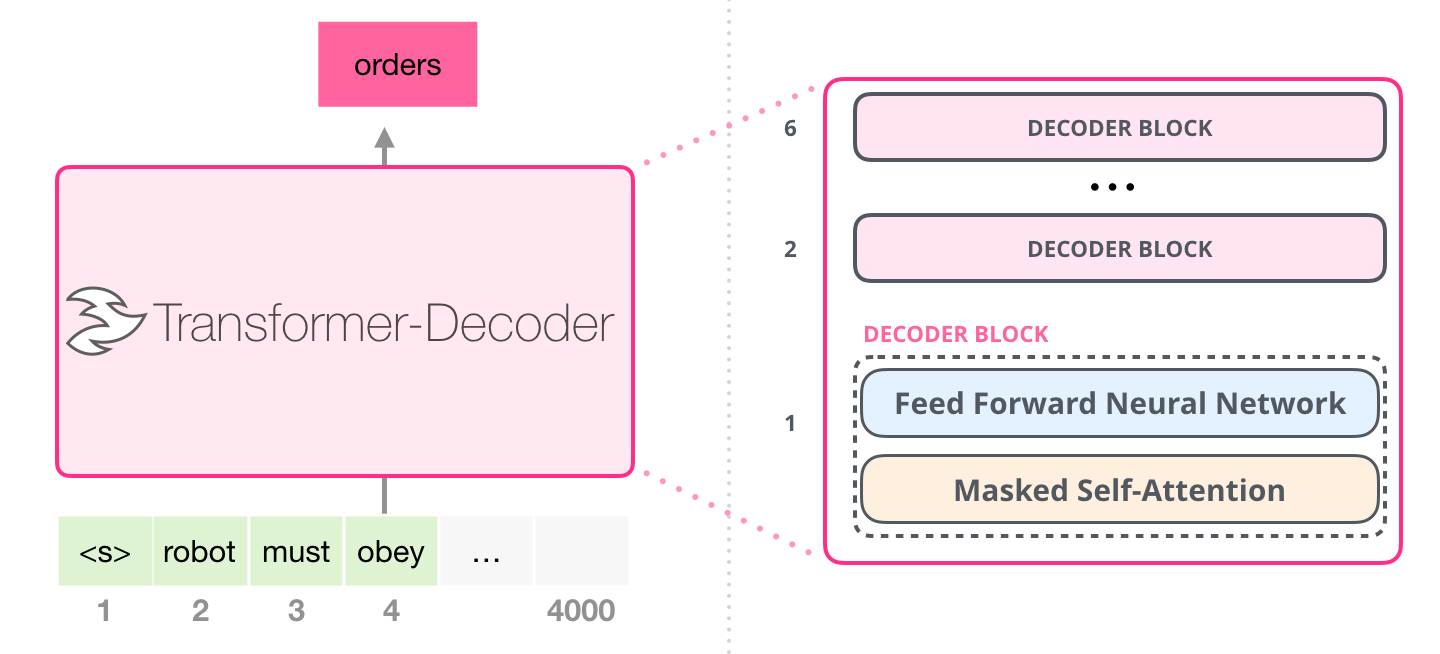
GPT(Generative Pre-trained Transformer)基于Transformer解码器自回归地预测下一个Token,从而进行了语言模型的建模。
只要能够足够好地预测下一个Token,语言模型便可能具备足够地潜力,从而实现人工智能。
以上就是关于GPT和它的能力的一个高层次概述。让我们深入了解更多具体细节。
输入 / 输出
GPT的函数签名大致如下:
def gpt(inputs: list[int]) -> list[list[float]]:
	""" GPT代码,实现预测下一个token
	inputs:List[int], shape为[n_seq],输入文本序列的token id的列表
	output:List[List[int]], shape为[n_seq, n_vocab],预测输出的logits列表
	"""
    output = # 需要实现的GPT内部计算逻辑
    return output
输入
输入是一些由整数表示的文本序列,每个整数都与文本中的token一一对应。例如:
text  = "robot must obey orders"
tokens = ["robot", "must", "obey", "orders"]
inputs = [1, 0, 2, 4]
token, 即词元,是文本的子片段,使用某种分词器生成。
分词器将文本分割为不可分割的词元单位,实现文本的高效表示,且方便模型学习文本的结构和语义。
分词器对应一个词汇表,我们可用词汇表将token映射为整数:
# 词汇表中的token索引表示该token的整数ID
# 例如,"robot"的整数ID为1,因为vocab[1] = "robot"
vocab = ["must", "robot", "obey", "the", "orders", "."]

# 一个根据空格进行分词的分词器tokenizer
tokenizer = WhitespaceTokenizer(vocab)

# encode()方法将str字符串转换为list[int]
ids = tokenizer.encode("robot must obey orders") # ids = [1, 0, 2, 4]

# 通过词汇表映射,可以看到实际的token是什么
tokens = [tokenizer.vocab[i] for i in ids] # tokens = ["robot", "must", "obey", "orders"]

# decode()方法将list[int] 转换回str
text = tokenizer.decode(ids) # text = "robot must obey orders"
简而言之:
- 通过语料数据集和分词器tokenizer可以构造一个包含文本中的所有token的词汇表vocab。
- 使用tokenizer将文本text分割为token序列,再使用词汇表vocab将token映射为token id整数,从而得到输入文本token序列。
最后,可以通过vocab将token id序列再转换回文本。
输出
output是一个二维数组,其中output[i][j]表示文本序列的第i个位置的token(inputs[i])是词汇表的第j个token(vocab[j])的概率(实际为未归一化的logits得分)。例如:
inputs = [1, 0, 2, 4]  # "robot" "must" "obey" "orders"
vocab = ["must", "robot", "obey", "the", "orders", "."]
output = gpt(inputs)

# output[0] = [0.75, 0.1, 0.15, 0.0, 0.0, 0.0]
# 给定 "robot",模型预测 "must" 的概率最高

# output[1] = [0.0, 0.0, 0.8, 0.1, 0.0, 0.1]
# 给定序列 ["robot", "must"],模型预测 "obey" 的概率最高

# output[-1] = [0.0, 0.0, 0.1, 0.0, 0.85, 0.05]
# 给定整个序列["robot", "must", "obey"],模型预测 "orders" 的概率最高
next_token_id = np.argmax(output[-1])  # next_token_id = 4
next_token = vocab[next_token_id]      # next_token = "orders"
在上述例子中,输入序列为["robot", "must", "obey"],GPT模型根据输入,预测序列的下一个token是 "output",因为 output[-1][4]的值为0.85,是词表中最高的一个。
- output[0] 表示给定输入token "robot",模型预测下一个token可能性最高的是"must",为0.75。
- output[-1] 表示给定整个输入序列 ["robot", "must", "obey"],模型预测下一个token是"orders"的可能性最高,为0.85。
为预测序列的下一个token,只需在output的最后一个位置中选择可能性最高的token。那么,通过迭代地将上一轮的输出拼接到输入,并送入模型,从而持续地生成token。
这种生成方式称为贪心采样。实际可以对类别分布用温度系数T进行蒸馏(放大或减小分布的不确定性),并截断类别分布的按top-k,再进行类别分布采样。
具体地,在每次迭代中,将上一轮预测出的token添加到输入末尾,然后预测下一个位置的值,如此往复,就是整个自回归的预测过程:
def generate(inputs, n_tokens_to_generate):
	""" GPT生成代码
	inputs: list[int], 输入文本的token ids列表
	n_tokens_to_generate:int, 需要生成的token数量
	"""
    # 自回归式解码循环
    for _ in range(n_tokens_to_generate):
        output = gpt(inputs)            # 模型前向推理,输出预测词表大小的logits列表
        next_id = np.argmax(output[-1]) # 贪心采样
        inputs.append(int(next_id))     # 将预测添加回输入
    return inputs[len(inputs) - n_tokens_to_generate :]  # 只返回生成的ids

# 随便举例
input_ids = [1, 0, 2]                          # ["robot", "must", "obey"]
output_ids = generate(input_ids, 1)            #  output_ids = [1, 0, 2, 4]
output_tokens = [vocab[i] for i in output_ids] # ["robot", "must", "obey", "orders"]
二、GPT结构与实现
2.1 基本组成部分
首先,导入相关可视化函数
import random
import numpy as np
import matplotlib.pyplot as plt

def plot(x, y, x_axis=None, y_axis=None):
    plt.plot(x, y)
    if x_axis and isinstance(x_axis, tuple):
        plt.xlim(x_axis[0], x_axis[1])
    if y_axis and isinstance(y_axis, tuple):
        plt.ylim(y_axis[0], y_axis[1])
    plt.show()

def plotHot(w):
    plt.figure()
    plt.imshow(w, cmap='hot', interpolation='nearest')
    plt.show()
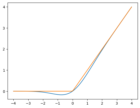
GELU
GPT-2选择的FFN中的非线性激活函数是GELU(高斯误差线性单元),是ReLU的对比的一种替代方法。它由以下函数近似表示:
def gelu(x):
    return 0.5 * x * (1 + np.tanh(np.sqrt(2 / np.pi) * (x + 0.044715 * x**3)))

def relu(x):
    return np.maximum(0, x)
GELU与ReLU的对比
print(gelu(np.array([1, 2, -2, 0.5])))
print(relu(np.array([1, 2, -2, 0.5])))

x = np.linspace(-4, 4, 100)
plot(x, np.array([gelu(x), relu(x)]).transpose())
Softmax
原始Softmax公式:$$\text{softmax}(x)_i = \frac{e^{x_i}}{\sum_j e^{x_j}}$$
相比原始Softmax, 这里使用了减去最大值max(x)技巧来保持数值稳定性。
def softmax(x):
    # 减去最大值,避免溢出,不影响分布
    exp_x = np.exp(x - np.max(x, axis=-1, keepdims=True))
    return exp_x / np.sum(exp_x, axis=-1, keepdims=True)

def rawSoftmax(x):
    exp_x = np.exp(x)
    return exp_x / np.sum(exp_x)
num = 100  # 生成不重复的随机数,比较 原始值、原始softmax和修正后的softmax
numbers = []
for i in range(num):
    number = random.uniform(1, 3)
    while number in numbers:
        number = random.uniform(1, 3)
    numbers.append(number)
plot(np.array(range(num)), np.array([numbers, rawSoftmax(numbers), softmax(numbers)]).transpose())
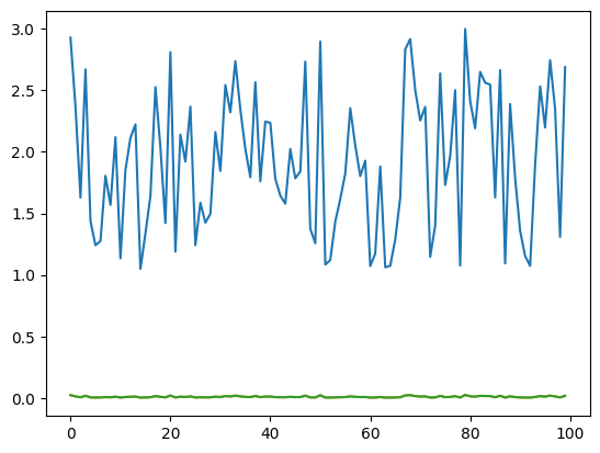
在输入在合理范围时,两者输出基本相同。
raw_x = np.array([[-200, 100, -300, 0, 70000000]])
x1 = softmax(raw_x)
x2 = rawSoftmax(np.array(raw_x))
print(x1, x1.sum(axis=-1), softmax(x1))
print(x2, x2.sum(axis=-1), softmax(x2))
在输入存在异常值时,输出结果比较(原始softmax出现nan)
[[0. 0. 0. 0. 1.]] [1.] [[0.14884758 0.14884758 0.14884758 0.14884758 0.40460968]]
[[ 0.  0.  0.  0. nan]] [nan] [[nan nan nan nan nan]]
tmp.py:7: RuntimeWarning: overflow encountered in exp exp_x = np.exp(x)
tmp.py:8: RuntimeWarning: invalid value encountered in divide return exp_x / np.sum(exp_x)
层归一化
层归一化(Layer Normalization)是基于特征维度将数据进行标准化(均值为0方差为1),同时乘以缩放系数、加上平移系数,保留其非线性能力:
层归一化可以有效地缓解优化过程中潜在的不稳定、收敛速度慢等问题。
def layer_norm(x, g, b, eps: float = 1e-5):
    """ 层归一化操作
    x: np.array, 输入
    g: float, 可学习的缩放参数 gamma
    b: float, 可学习的平移参数 beta
	eps: float, 避免方差为0从而除零的极小值
    """
    mean = np.mean(x, axis=-1, keepdims=True)
    variance = np.var(x, axis=-1, keepdims=True)
    x = (x - mean) / np.sqrt(variance + eps)  # 将x沿着最后一个轴,进行标准化
    return g * x + b                          # 将标准化后的x进行重新缩放和平移
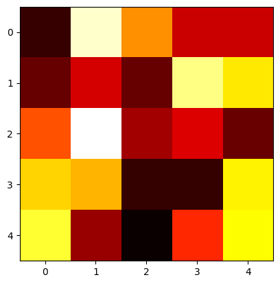
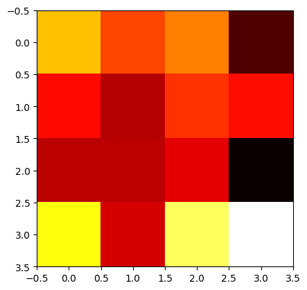
可视化例子
num, dim = 5, 5
x = np.array([[random.randint(-10, 10) for _ in range(dim)] for _ in range(num)] )
g, b = 1, 0 # 不缩放和平移
x_norm = layer_norm(x, g, b)
print(x)
print(x_norm)
plotHot(x)
plotHot(x_norm)
输出结果
# 层归一化前
[[ -9   3  -2  -6  -6]
 [-10  -6 -10   8   4]
 [ -1   5  -4  -3  -5]
 [  8   7  -5  -5   9]
 [ 10  -1  -5   3   9]]

# 层归一化后
[[-1.2056067   1.68784939  0.48224268 -0.48224268 -0.48224268]
 [-0.96768591 -0.43008263 -0.96768591  1.45152886  0.91392558]
 [ 0.16876312  1.8563943  -0.67505247 -0.39378061 -0.95632434]
 [ 0.8124999   0.65624992 -1.21874985 -1.21874985  0.96874988]
 [ 1.18444594 -0.73156955 -1.42830246 -0.03483665  1.01026272]]
层归一化前
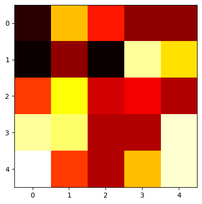
层归一化后(每行数据经过标准化后,分布差异变小了,从而输入网络的数据的分布得到了限制)
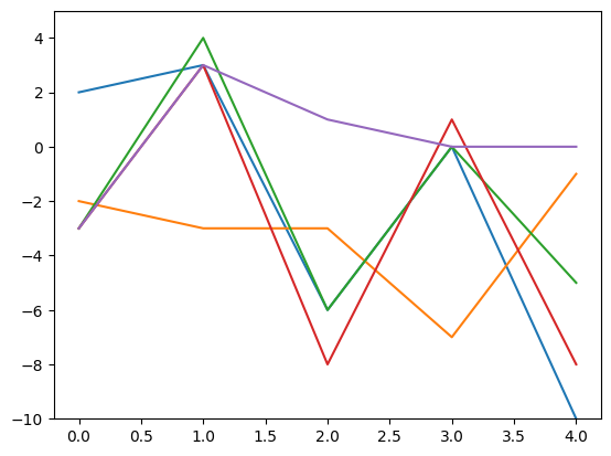
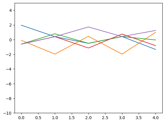
通过折线图可视化(每条折线代表一个行向量),可以更明显地看到变化:
axis = np.array(range(x.shape[0]))
plot(axis, x)
plot(axis, x_norm)
层归一化前
层归一化后
线性(仿射变换)层
标准的矩阵乘法+偏置:
def linear(x, w, b):  # [m, in], [in, out], [out] -> [m, out]
    return x @ w + b
例子
n_num = 3
in_dim, hid_dim = 4, 4
x = np.random.normal(size=(n_num, in_dim))
w = np.random.normal(size=(in_dim, hid_dim))
b = np.random.normal(size=(hid_dim,))
h = linear(x, w, b)
print(f"shape of w: {w.shape}")
print(f"input shape: {x.shape}, output shape: {h.shape}")
plotHot(w)
shape of w: (4, 4)
input shape: (3, 4), output shape: (3, 4)
权重可视化
2.2 GPT架构
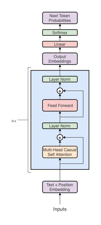
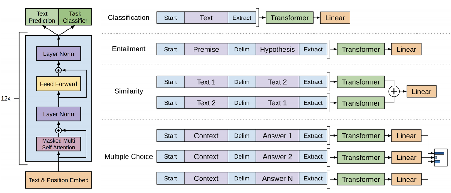
从整体上来看,GPT架构分为三个部分:
- 嵌入表示层:文本词元嵌入(token embeddings) + 位置嵌入(positional embeddings)
- transformer解码器堆栈:多层decoder block堆叠
- 预测:输出投影回词汇表(projection to vocab)
代码层GPT实现
def gpt2(inputs, wte, wpe, blocks, ln_f, n_head):
    """ GPT2模型实现
        输入输出tensor形状: [n_seq] -> [n_seq, n_vocab]
        n_vocab, 词表大小
        n_seq, 输入token序列长度
        n_layer, 自注意力编码器的层数
        n_embd, 词表的词元嵌入大小
        n_ctx, 输入最大序列长度(位置编码支持的长度,可用ROPE旋转位置编码提升外推长度)
    params:
        inputs: List[int], token ids, 输入token ids
        wte: np.ndarray[n_vocab, n_embd], token嵌入矩阵 (与输出分类器共享参数)
        wpe: np.ndarray[n_ctx, n_embd], 位置编码嵌入矩阵
        blocks:object, n_layer层因果自注意力编码器
        ln_f:tuple[float], 层归一化参数
        n_head:int, 注意力头数
    """
    # 1、在词元嵌入中添加位置编码信息:token + positional embeddings
    x = wte[inputs] + wpe[range(len(inputs))]  # [n_seq] -> [n_seq, n_embd]

    # 2、前向传播n_layer层Transformer blocks
    for block in blocks:
        x = transformer_block(x, **block, n_head=n_head)  # [n_seq, n_embd] -> [n_seq, n_embd]

    # 3、Transformer编码器块的输出投影到词汇表概率分布上
    # 预测下个词在词表上的概率分布[ 输出语言模型的建模的条件概率分布p(x_t|x_t-1 ... x_1) ]
    x = layer_norm(x, **ln_f)  # [n_seq, n_embd] -> [n_seq, n_embd]
    # 就是和嵌入矩阵进行内积(编码器块的输出相当于预测值,内积相当于求相似度最大的词汇)
    return x @ wte.T  # [n_seq, n_embd] -> [n_seq, n_vocab]
嵌入表示层
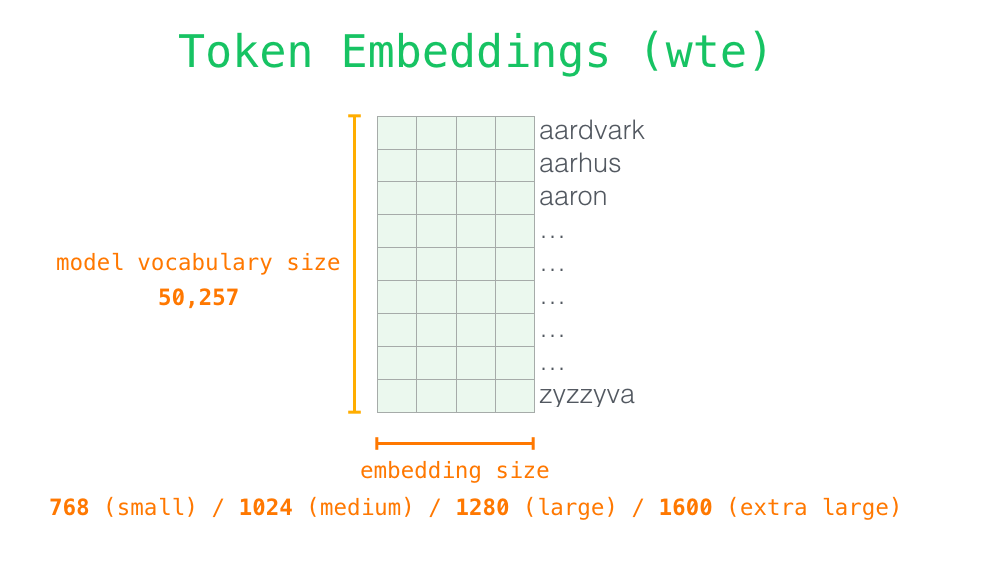
Token embeddings
wte是一个[n_vocab, n_embd]可学习参数矩阵,它充当一个token嵌入查找表,其中矩阵的第\(i\)
行对应于我们词汇表中第 \(i\)个token的embedding。
wte[inputs] 使用整数数组索引来检索与输入中每个token对应的向量。
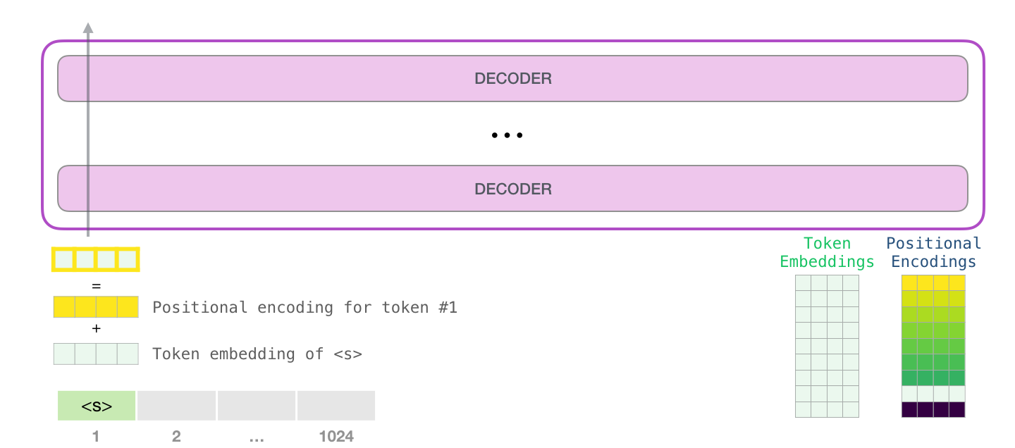
Positional embeddings
为了编码序列的顺序信息,通过在输入表示中添加位置编码(positional encoding)嵌入来注入位置信息。
位置编码可以通过学习得到也可以直接固定得到。
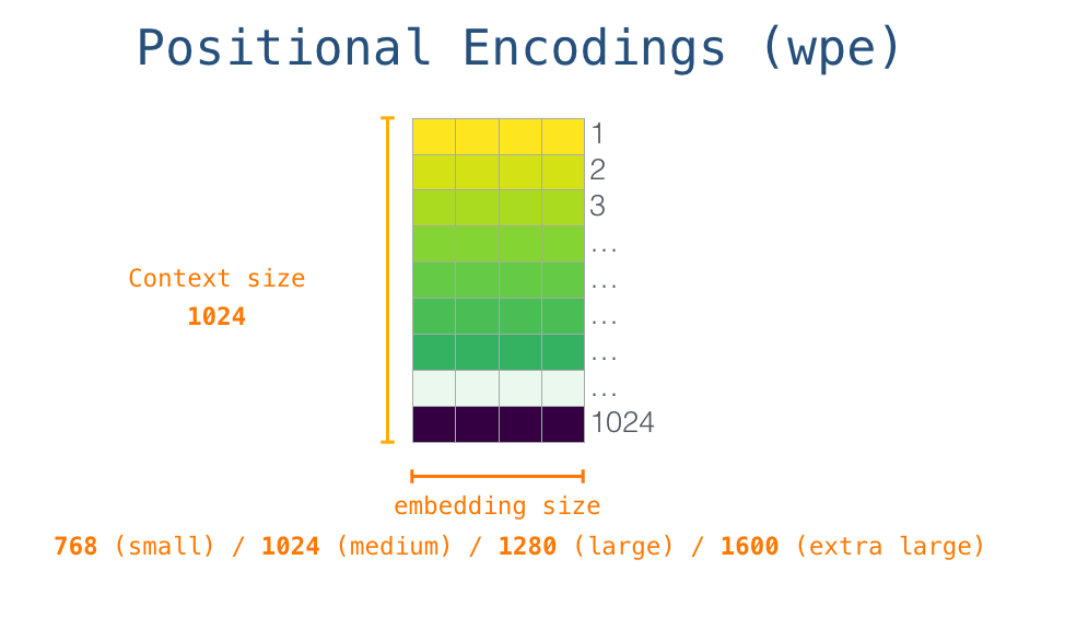
大小为[n_ctx, n_embd]的wpe即可学习的位置嵌入矩阵,其中矩阵的第\(i\)行对应输入序列中第\(i\)个token的位置embedding,编码了对应的位置信息。
n_ctx代表最大序列长度,限制了模型外推的最大范围。n_ctx代表最大序列长度,限制了模型外推的最大范围。
在GPT中,位置嵌入矩阵wpe和token embeddings类似,先随机初始化,后通过训练学习得到。wpe[inputs] 使用整数数组索引inputs来检索与输入中每个token对应的位置嵌入。
将token嵌入与位置嵌入联合为一个组合嵌入,这个嵌入将token信息和位置信息都编码进来了。
Token + Positional embeddings
将Tokene mbeddings与位置嵌入拼接后的嵌入,将token信息和位置信息都编码进来了,它将作为transoformer decoder blocks的实际输入。
x = wte[inputs] + wpe[range(len(inputs))] # [n_seq] -> [n_seq, n_embd]
解码层
transformer解码器模块由两个子层组成:
- 多头因果自注意力(Multi-head causal self attention)
- 逐位置前馈神经网络(Position-wise feed forward neural network)
transformer解码器中,堆叠了num_layers个如下的transformer_block:
def transformer_block(x, mlp, attn, ln_1, ln_2, n_head):
    """ 自注意力编码器层实现 (只实现逻辑,各个子模块参数需传入)
        输入输出tensor形状: [n_seq, n_embd] -> [n_seq, n_embd]
        n_seq, 输入token序列长度
        n_embd, 词表的词元嵌入大小
    params:
        x: np.ndarray[n_seq, n_embd], 输入token嵌入序列
        mlp: object, 前馈神经网络
        attn: object, 注意力编码器层
        ln1: object, 线性层1
        ln2: object, 线性层2
        n_head:int, 注意力头数
    """
    # Multi-head Causal Self-Attention (层归一化 + 多头自注意力 + 残差连接 )
    x = x + mha(layer_norm(x, **ln_1), **attn, n_head=n_head)  # [n_seq, n_embd] -> [n_seq, n_embd]

    # Position-wise Feed Forward Network
    x = x + ffn(layer_norm(x, **ln_2), **mlp)  # [n_seq, n_embd] -> [n_seq, n_embd]

    return x
Self-Attention中的层规一化和残差连接用于提升训练的稳定性。
残差连接
残差连接引入输入直接到输出的通路,便于梯度回传从而缓解在优化过程中由于网络过深引起的梯度消失问题。
位置感知的前馈网络
对序列中的所有位置的表示进行变换时使用的是同一个2层隐藏层的MLP,故称其为position-wise的前馈网络(Position-wise Feed Forward Network)。
def ffn(x, c_fc, c_proj):
    """ 2层前馈神经网络实现 (只实现逻辑,各个子模块参数需传入)
        输入输出tensor形状: [n_seq, n_embd] -> [n_seq, n_embd]
        n_seq, 输入token序列长度
        n_embd, 词表的词元嵌入大小
        n_hid, 隐藏维度
    params:
        x: np.ndarray[n_seq, n_embd], 输入token嵌入序列
        c_fc: np.ndarray[n_embd, n_hid], 升维投影层参数, 默认:4*n_embd
        c_proj: np.ndarray[n_hid, n_embd], 降维投影层参数
    """
    # project up:将n_embd投影到一个更高的维度 4*n_embd
    a = gelu(linear(x, **c_fc))  # [n_seq, n_embd] -> [n_seq, 4*n_embd]

    # project back down:投影回n_embd
    x = linear(a, **c_proj)  # [n_seq, 4*n_embd] -> [n_seq, n_embd]

    return x
这里仅仅是升维再降维,具体地将n_embd投影到一个更高的维度4*n_embd,然后再将其投影回n_embd。
多头因果自注意力
这里将通过分别解释“多头因果自注意力”的每个词,来一步步理解“多头因果自注意力”:
- 注意力(Attention)
- 自(Self)
- 因果(Causal)
- 多头(Multi-Head)
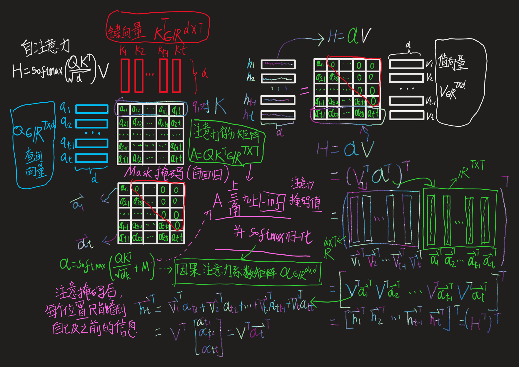
缩放点积注意力(scaled dot-product attention)
其中,查询向量\(\mathbf Q\in\mathbb R^{T\times d}\)、 键向量\(\mathbf K \in\mathbb R^{T\times d}\)、值向量\(\mathbf V\in\mathbb R^{T\times d}\),\(T\)为序列长度。
注意力得分除以\(\sqrt{d}\)进行缩放, 是考虑到在\(d\)过大时,点积值较大会使得后续Softmax操作溢出导致梯度爆炸,不利于模型优化。
def attention_raw(q, k, v):
    """ 原始缩放点积注意力实现
        输入输出tensor形状: [n_q, d_k], [n_k, d_k], [n_k, d_v] -> [n_q, d_v]
    params:
        q: np.ndarray[n_seq, n_embd], 查询向量
        k: np.ndarray[n_seq, n_embd], 键向量
        v: np.ndarray[n_seq, n_embd], 值向量
    """
    return softmax(q @ k.T / np.sqrt(q.shape[-1])) @ v

# 以通过对q、k、v进行投影变换来增强自注意效果
def self_attention_raw(x, w_k, w_q, w_v, w_proj):
    """ 自注意力原始实现
        输入输出tensor形状: [n_seq, n_embd] -> [n_seq, n_embd]
    params:
        x: np.ndarray[n_seq, n_embd], 输入token嵌入序列
        w_k: np.ndarray[n_embd, n_embd], 查询向量投影层参数
        w_q: np.ndarray[n_embd, n_embd], 键向量投影层参数
        w_v: np.ndarray[n_embd, n_embd], 值向量投影层参数
        w_proj: np.ndarray[n_embd, n_embd], 自注意力输出投影层参数
    """
    # qkv projections
    q = x @ w_k # [n_seq, n_embd] @ [n_embd, n_embd] -> [n_seq, n_embd]
    k = x @ w_q # [n_seq, n_embd] @ [n_embd, n_embd] -> [n_seq, n_embd]
    v = x @ w_v # [n_seq, n_embd] @ [n_embd, n_embd] -> [n_seq, n_embd]

    # perform self attention
    x = attention(q, k, v) # [n_seq, n_embd] -> [n_seq, n_embd]

    # out projection
    x = x @ w_proj # [n_seq, n_embd] @ [n_embd, n_embd] -> [n_seq, n_embd]

    return x

# 将w_q、w_k和w_v组合成一个单独的矩阵w_fc,执行投影操作,然后拆分结果,我们就可以将矩阵乘法的数量从4个减少到2个
def self_attention(x, c_attn, c_proj):
    """ 自注意力优化后实现(w_q 、w_k 、w_v合并成一个矩阵w_fc进行投影,再拆分结果)
        同时GPT-2的实现:加入偏置项参数(所以使用线性层,进行仿射变换)
        输入输出tensor形状: [n_seq, n_embd] -> [n_seq, n_embd]
    params:
        x: np.ndarray[n_seq, n_embd], 输入token嵌入序列
        w_fc: np.ndarray[n_embd, 3*n_embd], 查询向量投影层参数
        w_proj: np.ndarray[n_embd, n_embd], 自注意力输出投影层参数
    """
    # qkv projections
    x = linear(x, **c_attn) # [n_seq, n_embd] -> [n_seq, 3*n_embd]

    # split into qkv
    q, k, v = np.split(x, 3, axis=-1) # [n_seq, 3*n_embd] -> 3 of [n_seq, n_embd]

    # perform self attention
    x = attention(q, k, v) # [n_seq, n_embd] -> [n_seq, n_embd]

    # out projection
    x = linear(x, **c_proj) # [n_seq, n_embd] @ [n_embd, n_embd] = [n_seq, n_embd]

    return x
因果
为了防止序列建模时出现信息泄露,需要修改注意力矩阵(增加Mask)以隐藏或屏蔽我们的输入,从而避免模型在训练阶段直接看到后续的文本序列(信息泄露)进而无法得到有效地训练。
# 输入是 ["not", "all", "heroes", "wear", "capes"]

# 原始自注意力
        not    all   heroes  wear  capes
   not 0.116  0.159  0.055  0.226  0.443
   all 0.180  0.397  0.142  0.106  0.175
heroes 0.156  0.453  0.028  0.129  0.234
  wear 0.499  0.055  0.133  0.017  0.295
 capes 0.089  0.290  0.240  0.228  0.153

 # 因果自注意力 (行为j, 列为i)
 # 为防止输入的所有查询都能预测未来,需要将所有j>i位置设置为0 :
        not    all   heroes  wear  capes
   not 0.116  0.     0.     0.     0.
   all 0.180  0.397  0.     0.     0.
heroes 0.156  0.453  0.028  0.     0.
  wear 0.499  0.055  0.133  0.017  0.
 capes 0.089  0.290  0.240  0.228  0.153

 # 在应用 softmax 之前,我们需要修改我们的注意力矩阵,得到掩码自注意力
 # 即,在softmax之前将要屏蔽项的注意力得分设置为 −∞(归一化系数为0)
 # mask掩码矩阵
 0 -1e10 -1e10 -1e10 -1e10
 0   0   -1e10 -1e10 -1e10
 0   0     0   -1e10 -1e10
 0   0     0     0   -1e10
 0   0     0     0     0

 使用 -1e10 而不是 -np.inf ,因为 -np.inf 可能会导致 nans
加入掩码矩阵的注意力实现:
def attention(q, k, v, mask):
    """ 缩放点积注意力实现
        输入输出tensor形状: [n_q, d_k], [n_k, d_k], [n_k, d_v] -> [n_q, d_v]
    params:
        q: np.ndarray[n_seq, n_embd], 查询向量
        k: np.ndarray[n_seq, n_embd], 键向量
        v: np.ndarray[n_seq, n_embd], 值向量
        mask: np.ndarray[n_seq, n_seq], 注意力掩码矩阵
    """
    return softmax(q @ k.T / np.sqrt(q.shape[-1]) + mask) @ v
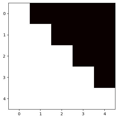
因果注意力掩码矩阵可视化
x = np.array([1, 1, 1, 1, 1])
causal_mask = (1 - np.tri(x.shape[0], dtype=x.dtype))* -1e10
print(causal_mask)
plotHot(causal_mask)
[[-0.e+00 -1.e+10 -1.e+10 -1.e+10 -1.e+10]
 [-0.e+00 -0.e+00 -1.e+10 -1.e+10 -1.e+10]
 [-0.e+00 -0.e+00 -0.e+00 -1.e+10 -1.e+10]
 [-0.e+00 -0.e+00 -0.e+00 -0.e+00 -1.e+10]
 [-0.e+00 -0.e+00 -0.e+00 -0.e+00 -0.e+00]]
注意力可视化
def causal_self_attention(x, c_attn, c_proj):
    """ 因果自注意力优化后实现(w_q 、w_k 、w_v合并成一个矩阵w_fc进行投影,再拆分结果)
        同时GPT-2的实现:加入偏置项参数(所以使用线性层,进行仿射变换)
        输入输出tensor形状: [n_seq, n_embd] -> [n_seq, n_embd]
    params:
        x: np.ndarray[n_seq, n_embd], 输入token嵌入序列
        c_attn: np.ndarray[n_embd, 3*n_embd], 查询向量投影层参数
        c_proj: np.ndarray[n_embd, n_embd], 自注意力输出投影层参数
    """
    # qkv projections
    x = linear(x, **c_attn) # [n_seq, n_embd] -> [n_seq, 3*n_embd]

    # split into qkv
    q, k, v = np.split(x, 3, axis=-1) # [n_seq, 3*n_embd] -> 3 of [n_seq, n_embd]

    # causal mask to hide future inputs from being attended to
    causal_mask = (1 - np.tri(x.shape[0], dtype=x.dtype))* -1e10   # [n_seq, n_seq]

    # perform causal self attention
    x = attention(q, k, v, causal_mask) # [n_seq, n_embd] -> [n_seq, n_embd]

    # out projection
    x = linear(x, **c_proj) # [n_seq, n_embd] @ [n_embd, n_embd] = [n_seq, n_embd]

    return x
实际,用-1e10替换-np.inf, 因为-np.inf会导致nans错误。
多头自注意力(Multi-Head-self-Attention)
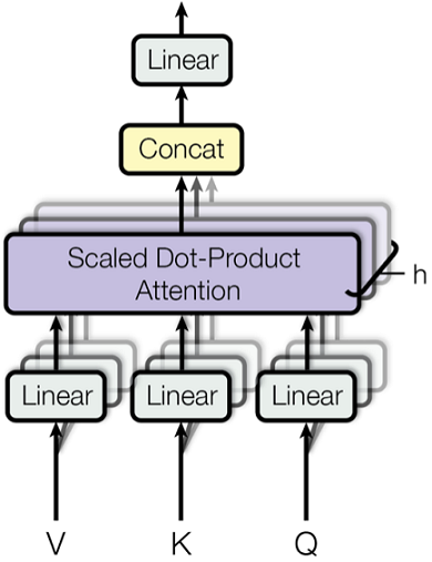
def mha(x, c_attn, c_proj, n_head):
    """ 多头自注意力实现
        输入输出tensor形状: [n_seq, n_embd] -> [n_seq, n_embd]
        每个注意力计算的维度从n_embd降低到 n_embd/n_head。
        通过降低维度,模型利用多个子空间进行建模
    params:
        x: np.ndarray[n_seq, n_embd], 输入token嵌入序列
        c_attn: np.ndarray[n_embd, 3*n_embd], 查询向量投影层参数
        c_proj: np.ndarray[n_embd, n_embd], 自注意力输出投影层参数
    """
    # qkv投影变换
    x = linear(x, **c_attn)  # [n_seq, n_embd] -> [n_seq, 3*n_embd]

    # 划分为qkv
    qkv = np.split(x, 3, axis=-1)  # [n_seq, 3*n_embd] -> [3, n_seq, n_embd]

    # 将n_embd继续划分为_head个注意力头
    qkv_heads = list(map(lambda x: np.split(x, n_head, axis=-1), qkv))  # [3, n_seq, n_embd] -> [3, n_head, n_seq, n_embd/n_head]

    # 构造causal mask矩阵
    causal_mask = (1 - np.tri(x.shape[0], dtype=x.dtype))* -1e10  # [n_seq, n_seq]

    # 单独执行每个头的因果自注意力(可多核多线程并行执行)
    out_heads = [attention(q, k, v, causal_mask) for q, k, v in zip(*qkv_heads)]  # [3, n_head, n_seq, n_embd/n_head] -> [n_head, n_seq, n_embd/n_head]

    # 合并多个heads的结果
    x = np.hstack(out_heads)  # [n_head, n_seq, n_embd/n_head] -> [n_seq, n_embd]

    # 多头因果自注意力输出projection
    x = linear(x, **c_proj)  # [n_seq, n_embd] -> [n_seq, n_embd]

    return x
将所有代码组合起来
将所有代码组合起来就得到了gpt2.py,总共的代码只有120行(如果你移除注释、空格之类的,那就只有60行)。
二、项目实战
可以通过以下代码测试:
python gpt2.py "Alan Turing theorized that computers would one day become" --n_tokens_to_generate 8
其输出是:the most powerful machines on the planet.
ToDO