Self-Supervised Hypergraph Convolutional Networks for Session-based Recommendation-526互联

Xia X., Yin H., Yu J., Wang Q., Cui L and Zhang X. Self-supervised hypergraph convolutional networks for session-based recommendation. AAAI, 2021.

概

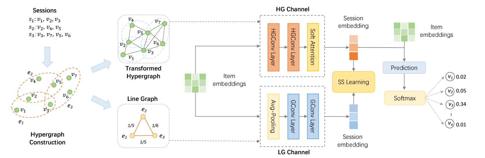
自监督加(超)图用于 session 推荐.
和 COTREC 简直就是双胞胎, 还是同一年发的, 还能这么玩啊.

\(I = \{i_1, i_2, i_3, \ldots, i_N\}\), items;
\(s = [i_{s,1}, i_{s, 2}, i_{s, 3}, \ldots, i_{s, m}]\), 某个 session 序列;
\(\mathbf{X}^{(l)} \in \mathbb{R}^{N \times d^{(l)}}\) 表示神经网络第 \(l\) 层的 embeddings, \(\mathbf{X}^{(0)}\) 为初始的 embeddings;

超图 \(G = (V, E)\), 其中 \(E\) 包含 \(M\) 条 hyperedges, 每条 hyperedge \(\epsilon \in E\) 可以包含多个结点, 其上的权重为 \(W_{\epsilon\epsilon}\). 由此可以得到对角矩阵:

\[\mathbf{W} \in \mathbb{R}^{M \times M}. \]
超图可以用 incidence matrix \(\mathbf{H} \in \mathbb{R}^{N \times M}\) 来表示, 其中 \(H_{i\epsilon} = 1\) 若 \(v_i \in \epsilon\).
由此, 我们可以构建 degree matrix:

\[\mathbf{D} = \text{diag}(\mathbf{HW}\mathbf{1}) \in \mathbb{R}^{N \times N}, \quad \mathbf{B} = \text{diag}(\mathbf{1}^T\mathbf{H}) \in \mathbb{R}^{M \times M}. \]

对于超图 \(G = (V, E)\), 定义它的 line graph 为 \(L(G) = (V_L, E_L)\), 其中的每个结点都是一条 hyperedge \(\epsilon\), 即 \(V_L = E\), 而:

\[E_L = \{(v_{e_p}, V_{e_q}): e_p, e_q \in E, |e_p \cap e_q| \ge 1\}. \]
文中对 \(E_L\) 中的每条边分配权重:

\[W_{p, q} = |e_p \cap e_q| / |e_p \cup e_q|. \]

这一步, 我们利用超图进行信息的传播:

\[\mathbf{X}_h^{(l+1)} = \underbrace{(\mathbf{D}^{-1}}_{E \rightarrow V} \mathbf{HW}) \underbrace{(\mathbf{B}^{-1} \mathbf{H}^T)}_{V \rightarrow E} \mathbf{X}_h^{(l)}, \]
这一步完成了 \(V \rightarrow E \rightarrow V\) 的信息聚合, 其中并没有可训练的参数.
接着, 融合各层的特征:

\[\mathbf{X}_h = \frac{1}{L+1} \sum_{l=0}^L \mathbf{X}_h^{(l)}. \]
注入位置信息:

\[\mathbf{x}_t^* = \tanh(\mathbf{W}_1[\mathbf{x}_t \| \mathbf{p}_{m-i+1}] + \mathbf{b}), \]
其中 \(\mathbf{W}_1 \in \mathbb{R}^{d \times 2d}, b \in \mathbb{R}^d\) 为可训练的参数,

\[\mathbf{P}_r = [\mathbf{p}_1, \mathbf{p}_2, \mathbf{p}_3, \ldots, \mathbf{p}_m]. \]
通过 soft attention 进行融合:

\[\theta_h = \sum_{t=1}^m \alpha_t \mathbf{x}_t, \\ \alpha_t = \mathbf{f}^T \sigma(\mathbf{W}_2 \mathbf{x}_s^* + \mathbf{W}_3 \mathbf{x}_t^* + \mathbf{c}), \\ \mathbf{x}_s^* = \frac{1}{m} \sum_{t=1}^m \mathbf{x}_m. \]
这一部分作为主要的 encoder, 用于推荐, 在训练中负责主要的推荐损失:

\[\mathcal{L}_r = -\sum_{i=1}^N \mathbf{y}_i \log (\mathbf{\hat{y}}_i) + (1 - \mathbf{y}_i) \log (1 - \mathbf{\hat{y}}_i), \\ \mathbf{\hat{y}} = \text{softmax}(\mathbf{\hat{z}}), \\ \mathbf{\hat{z}}_i = \theta_h^T \mathbf{x}_i. \\ \]

令 \(L(G)\) 的邻接矩阵表示为 \(\mathbf{A} = \in \mathbb{R}^{M \times M}, A_{p,q} = W_{p, q}\). \(\mathbf{\hat{A}} = \mathbf{A + I}\), \(\mathbf{\hat{D}}\) 为其 degree matrix, 则

\[\Theta_l^{(l+1)} = \mathbf{\hat{D}}^{-1} \mathbf{\hat{A}} \Theta^{(l)} \]
其中 \(\Theta^{(0)}\) 为 session 中 item embeddings 的平均.
接着, 采取 average 的方式进行融合:

\[\Theta_l = \frac{1}{L + 1} \sum_{l=0}^L \Theta_l^{(l)}. \]

我们视作 \((\theta_i^h, \theta_i^l)\) 为 postive pair, 而 \((\tilde{\theta}_i^h, \theta_i^l)\) 为 negative pair, 其中 \(\tilde{\theta}_i^h\) 是在 \(\Theta_h\) 进行 row-wise 和 col-wise shuffling 后得到的负样本.
接着, 我们用如下损失来鼓励 positive pair 接近, 而 negative pair 互相远离:

\[\mathcal{L}_s = -\log \sigma(f_D (\theta_i^h, \theta_i^l)) - \log \sigma(1 - f_D(\tilde{\theta}_i^h, \theta_i^l)). \]
这里, 我们用内积建模判别器 \(f_D\).