本文主要利用LSTM和CNN来处理移动传感器产生的数据识别人类活动。
传感器数据集
数据组成
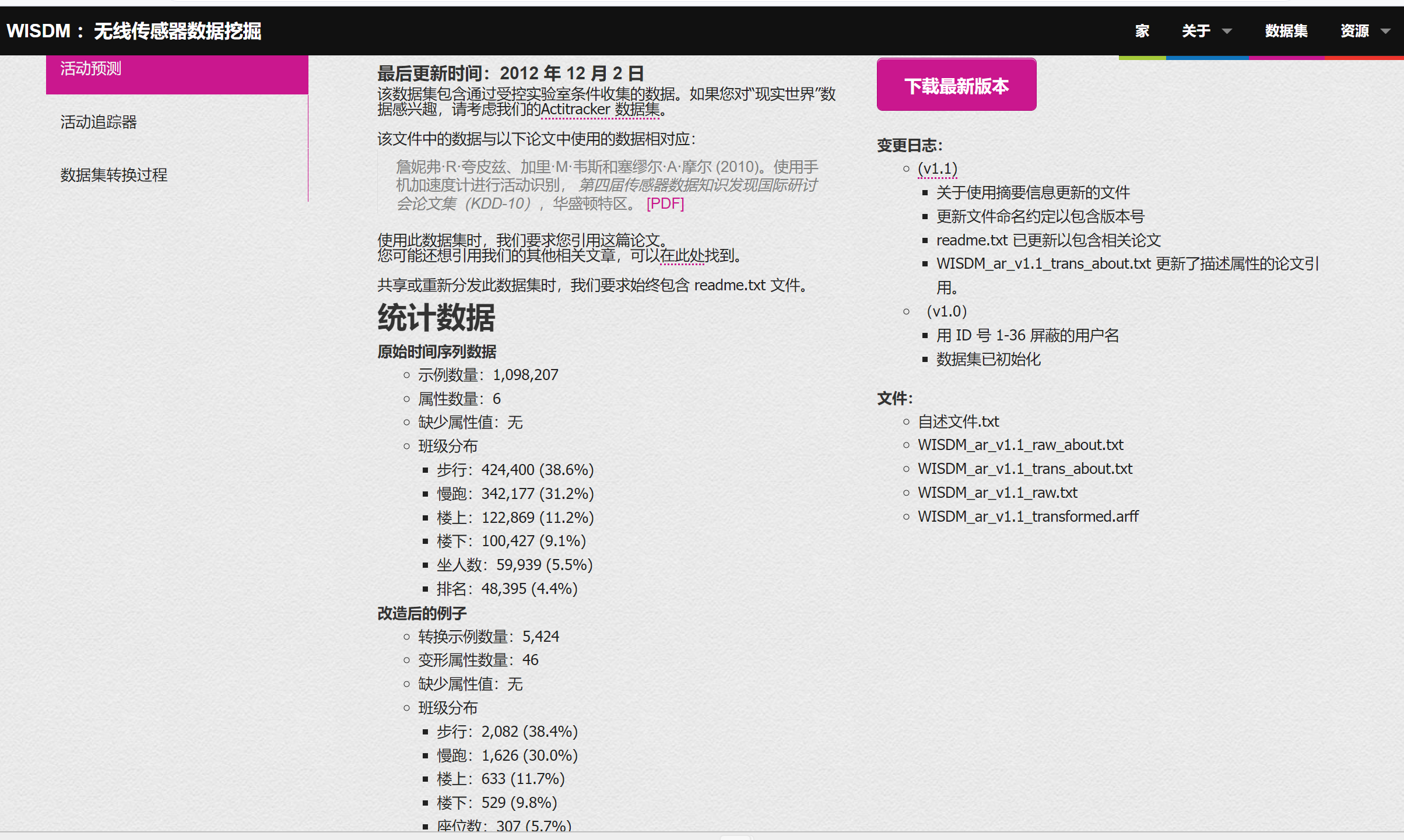
这个项目使用了 WISDM (Wireless Sensor Data Mining) Lab 实验室公开的 Actitracker 的数据集
其中数据:
测试记录:1,098,207 条
行为类型:6 种
- 走路
- 慢跑
- 上楼梯
- 下楼梯
- 坐
- 站立
传感器类型:加速度
测试场景:手机放在衣兜里面
WISDM 公开了两个数据集,一个是在实验室环境采集的;另一个是在真实使用场景中采集的,这里使用的是实验室环境采集的数据。
数据分析
其中数据又6中数据行为:
Walking -> 2,082 -> 38.4%,
Jogging -> 1,626 -> 30.0%,
Upstairs -> 633 -> 11.7%,
Downstairs -> 529 -> 9.8%,
Sitting -> 307 -> 5.7%,
Standing -> 247 -> 4.6%,
数据组成:
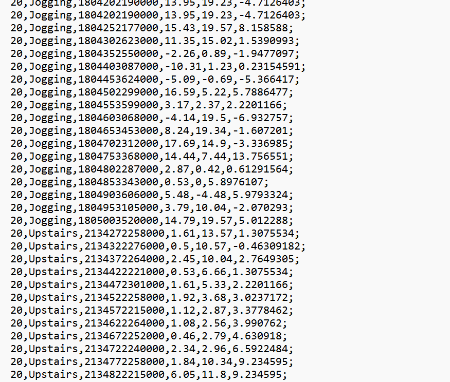
Raw.txt遵循以下格式:
[user-id],[activity],[timestamp],[x-acceleration],[y-accel],[z-accel]
- user-id 是用户的id:数据范围是[1..36]
- activity 是用户的行为,包括[Walking,Jogging,Upstairs,Downstairs,Sitting,Standing]
- timestamp 是用户手机里面的时间戳
- x-acceleration 是手机x轴的加速度,数值介于[-20,20]的浮点数
- y-accel 类似于x-accel
- z-accel 类似于z-accel
读取数据
column_names =['user-id', 'activity', 'timestamp', 'X', 'Y', 'Z']
df = pd.read_csv('Dataset/WISDM_ar_v1.1/WISDM_ar_v1.1_raw.txt',header=None, names=column_names)
df.head()
我们发现如果用上面的代码处理的话,会出现最后一行"Z"多了一个';'.
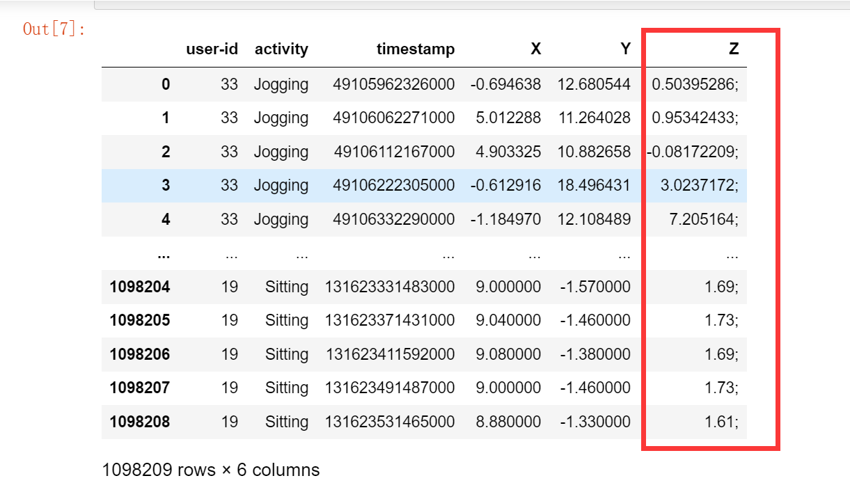
所以我们读取完了之后要处理一下
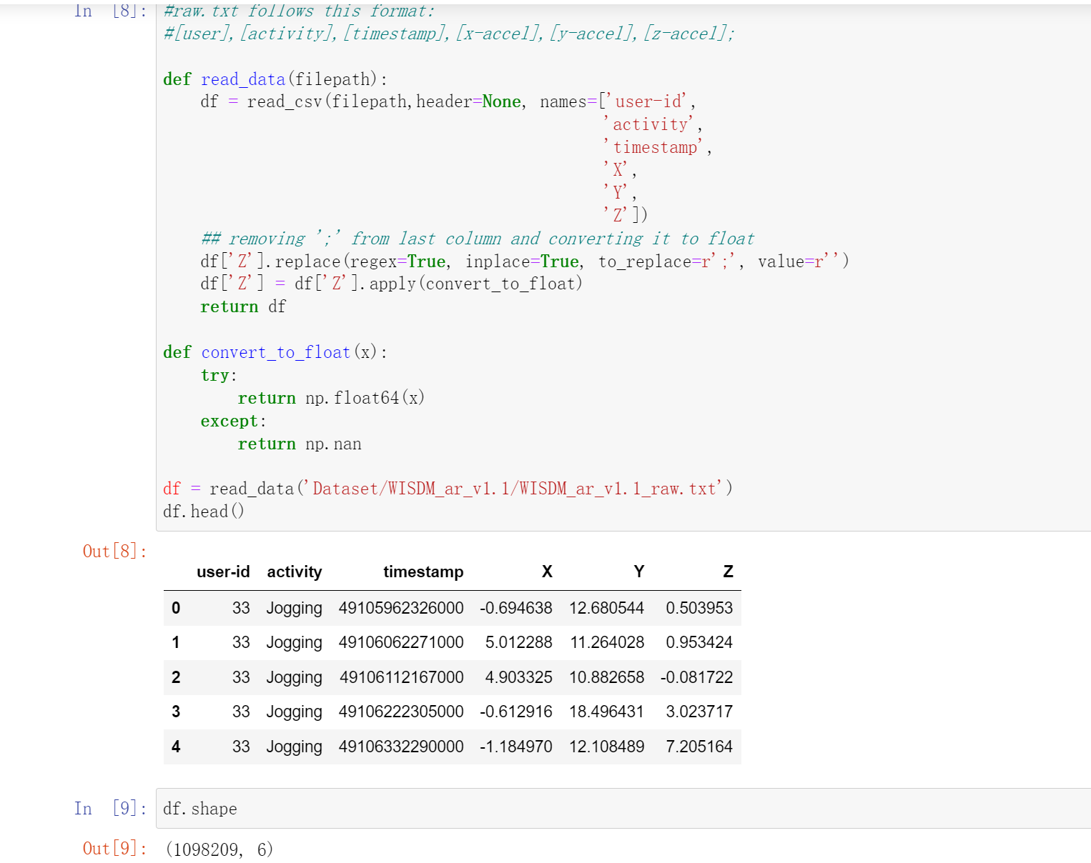
#raw.txt follows this format:
#[user],[activity],[timestamp],[x-accel],[y-accel],[z-accel];

def read_data(filepath):
    df = read_csv(filepath,header=None, names=['user-id',
                                               'activity',
                                               'timestamp',
                                               'X',
                                               'Y',
                                               'Z'])
    ## removing ';' from last column and converting it to float
    df['Z'].replace(regex=True, inplace=True, to_replace=r';', value=r'')
    df['Z'] = df['Z'].apply(convert_to_float)
    return df

def convert_to_float(x):
    try:
        return np.float64(x)
    except:
        return np.nan

df = read_data('Dataset/WISDM_ar_v1.1/WISDM_ar_v1.1_raw.txt')
df.head()
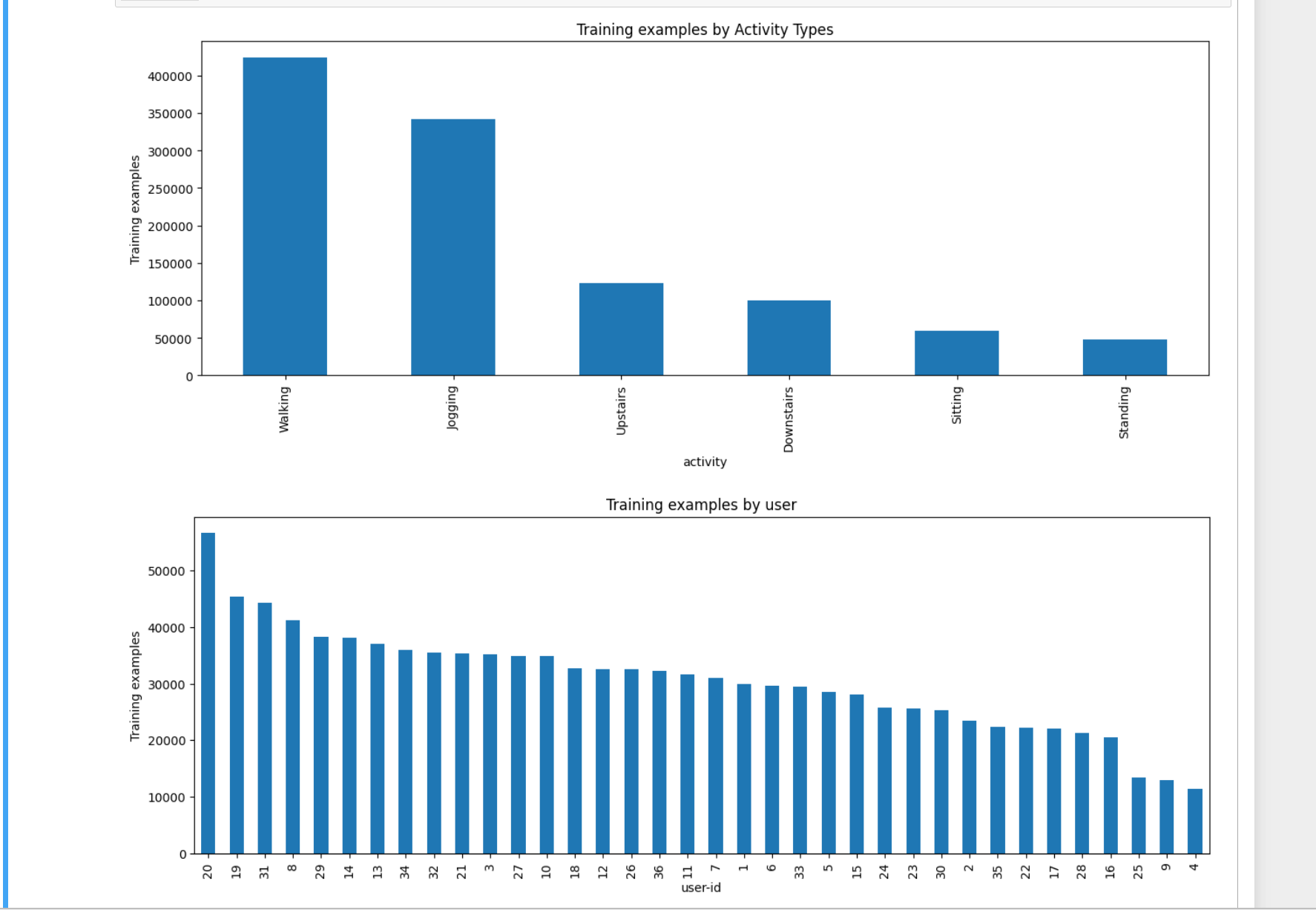
数据可视化分析
plt.figure(figsize=(15, 5))

plt.xlabel('Activity Type')
plt.ylabel('Training examples')
df['activity'].value_counts().plot(kind='bar',
                                  title='Training examples by Activity Types')
plt.show()

plt.figure(figsize=(15, 5))
plt.xlabel('User')
plt.ylabel('Training examples')
df['user-id'].value_counts().plot(kind='bar',
                                 title='Training examples by user')
plt.show()
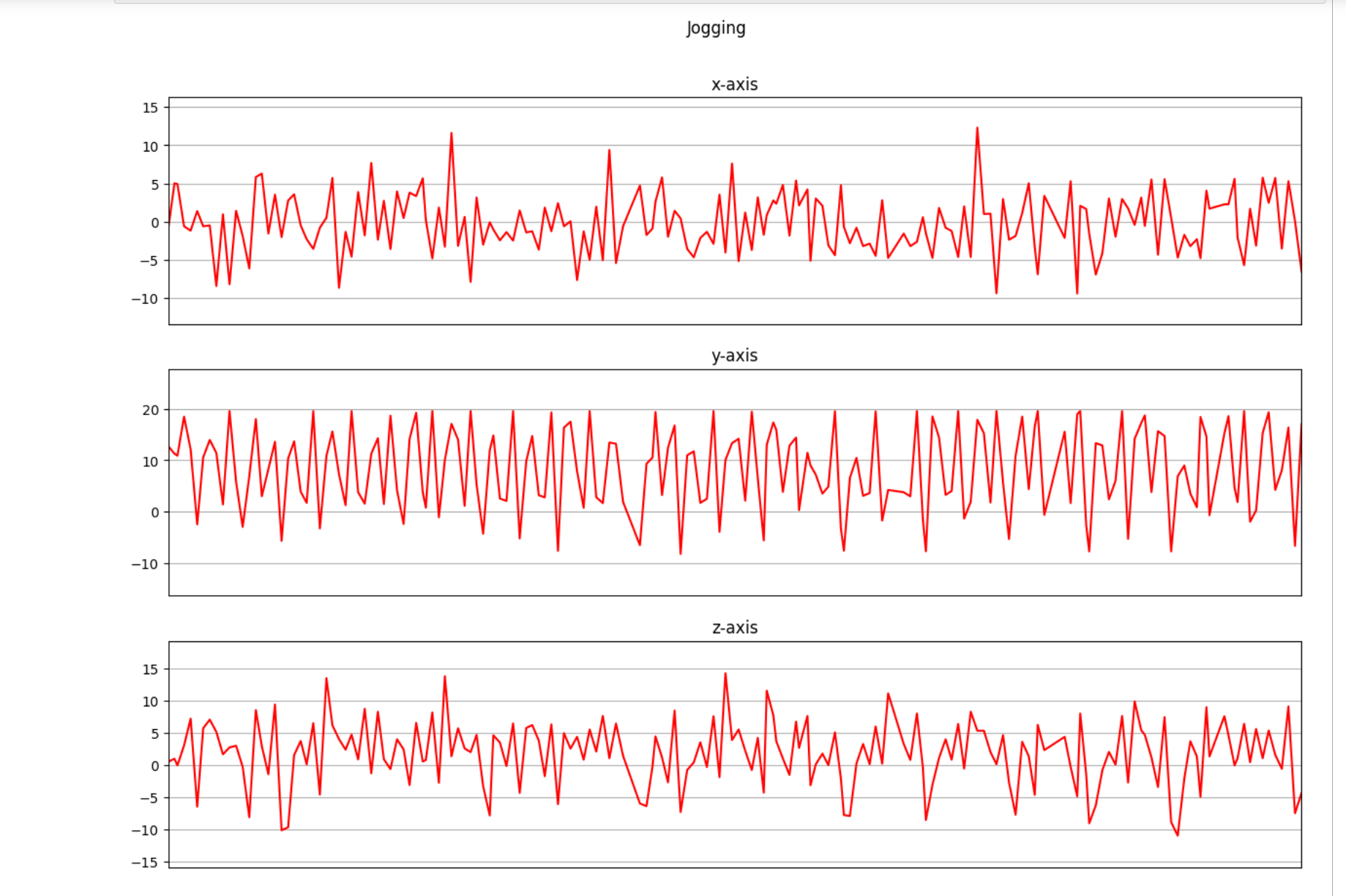
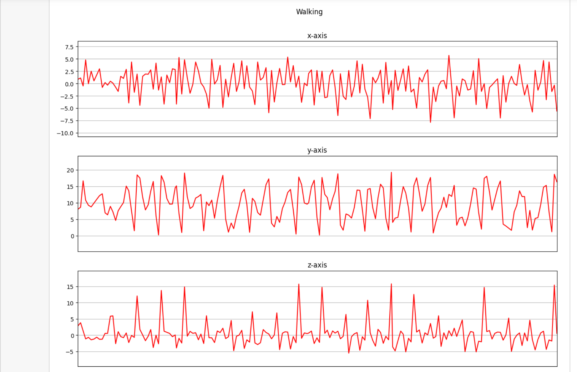
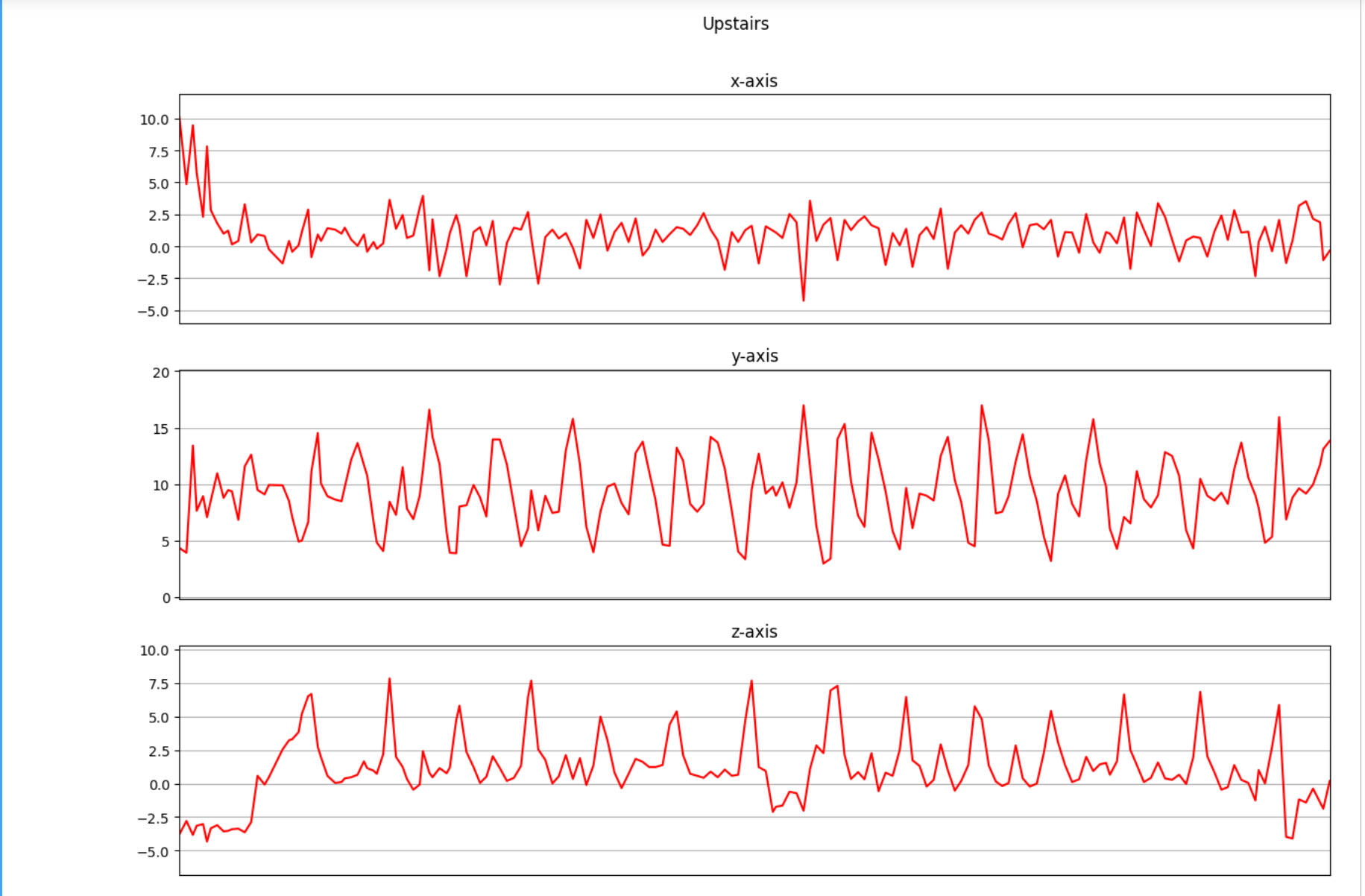
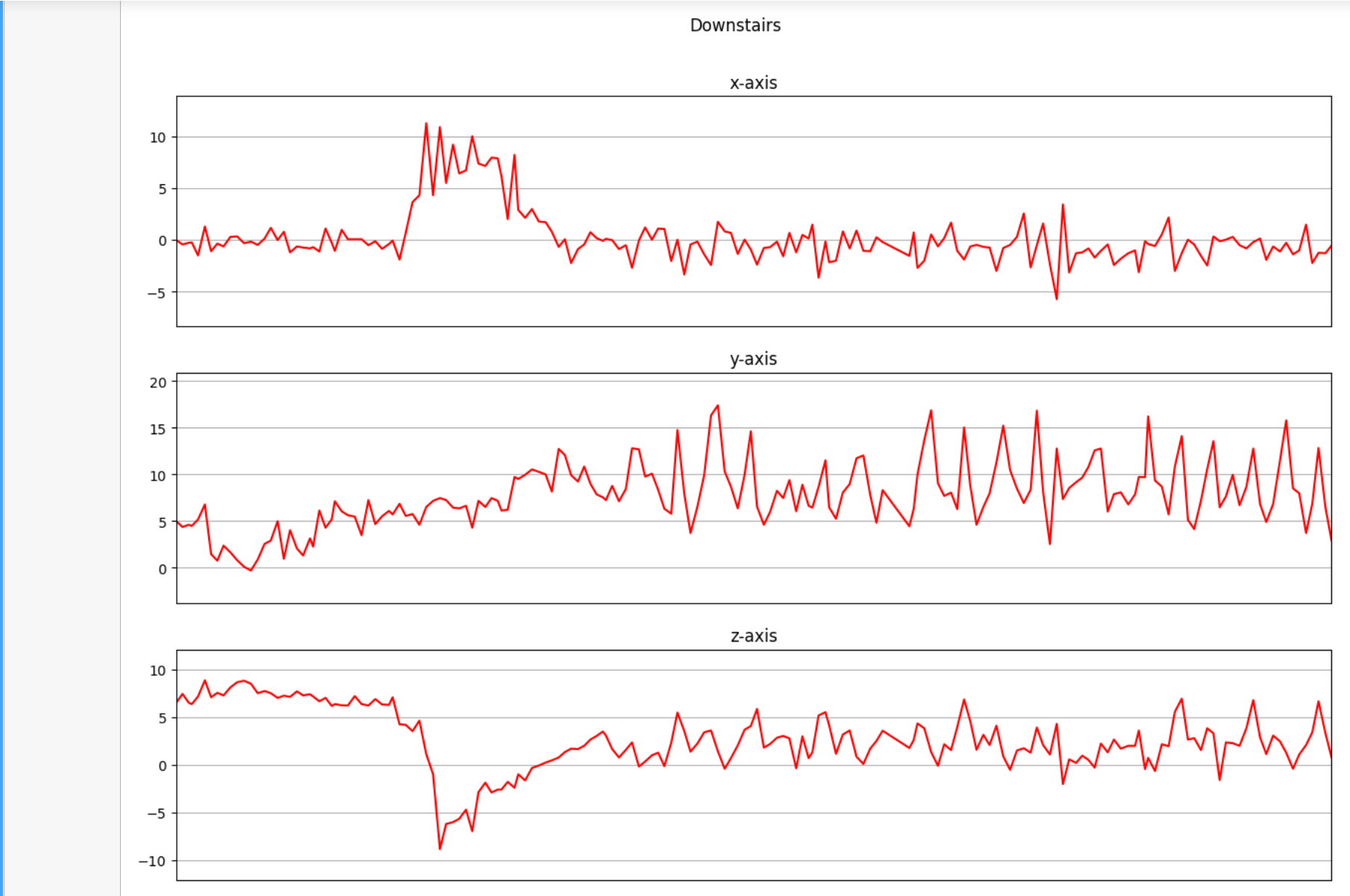
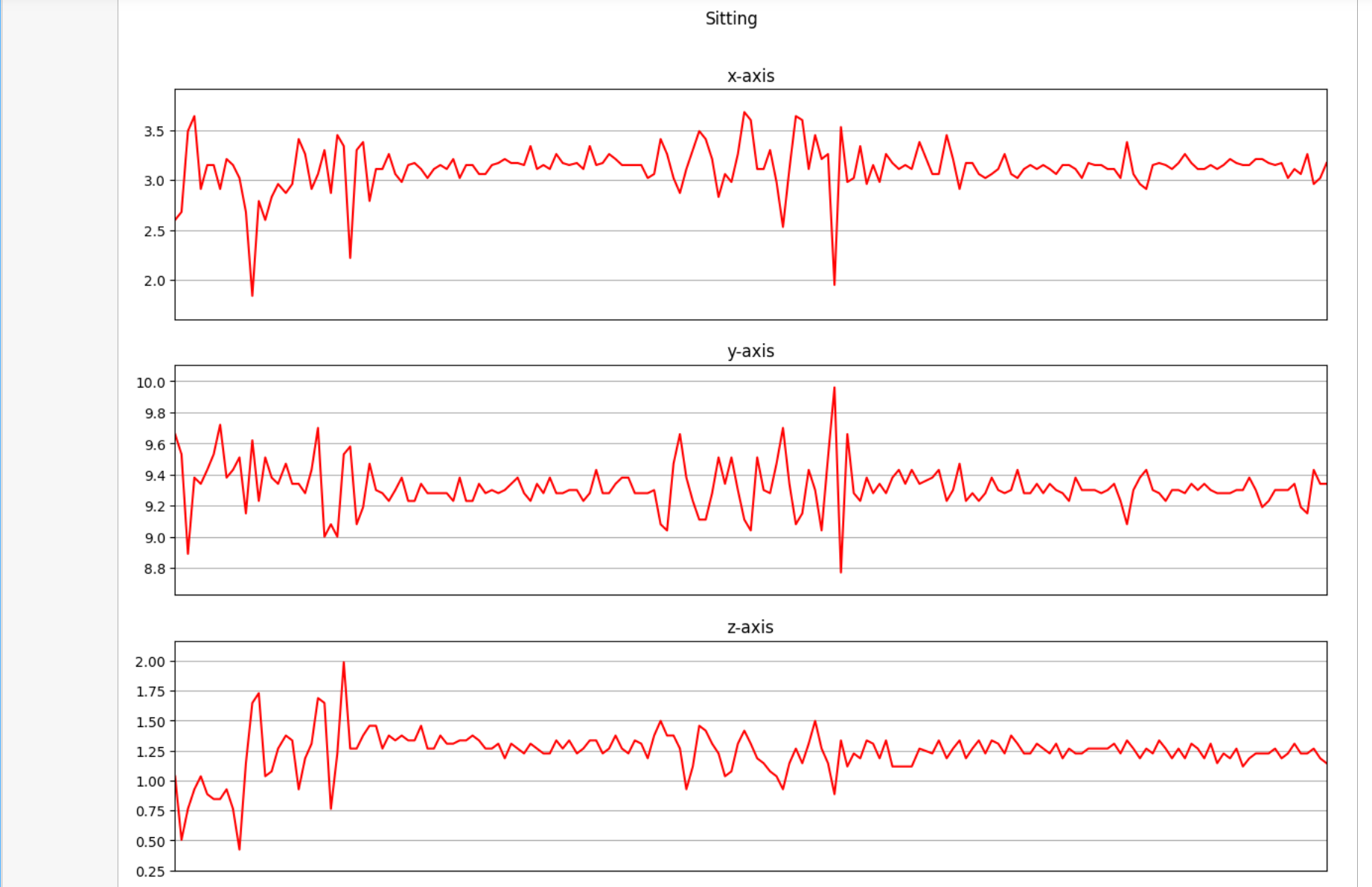
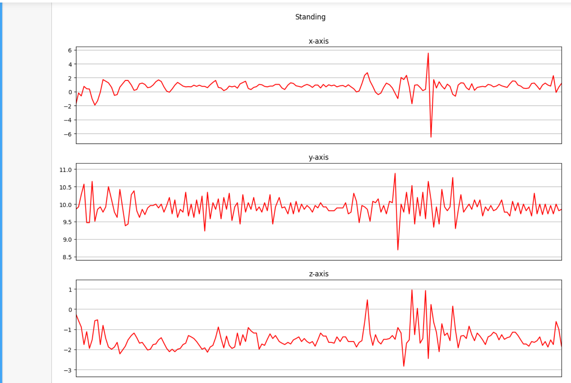
下面是我们将收集的三个轴上的加速度计数据进行可视化。
def axis_plot(ax, x, y, title):
    ax.plot(x, y, 'r')
    ax.set_title(title)
    ax.xaxis.set_visible(False)
    ax.set_ylim([min(y) - np.std(y), max(y) + np.std(y)])
    ax.set_xlim([min(x), max(x)])
    ax.grid(True)

for activity in df['activity'].unique():
    limit = df[df['activity'] == activity][:180]
    fig, (ax0, ax1, ax2) = plt.subplots(nrows=3, sharex=True, figsize=(15, 10))
    axis_plot(ax0, limit['timestamp'], limit['X'], 'x-axis')
    axis_plot(ax1, limit['timestamp'], limit['Y'], 'y-axis')
    axis_plot(ax2, limit['timestamp'], limit['Z'], 'z-axis')
    plt.subplots_adjust(hspace=0.2)
    fig.suptitle(activity)
    plt.subplots_adjust(top=0.9)
    plt.show()
数据预处理
其中包括:
- 标签编码
- 线性插值
- 数据分割
- 归一化
- 时间序列分割
- 独热编码
标签编码
因为我们的模型不接收数字标签,作为输入。由于我们是对这些行文进行预测,我们的预测结果可以是这些行为对应的数字标签。所以我们在原始数据中添加一列'activityEncode',来对应我们的每个行为。便于预测。这里有点类似于哈希,就是把每一个类别哈希成一个数字
Downstairs [0]
Jogging [1]
Sitting [2]
Standing [3]
Upstairs [4]
Walking [5]
这里遇到的API:是sklearn.preprocessing中的fit_transfrom ,官网
from sklearn.preprocessing import LabelEncoder
la = LabelEncoder()
la.fit([,,,])
Fit label encoder and return encoded labels.
Parameters:
yarray-like of shape (n_san_samples,)
Target values.
Returns:
yarray-like of shape (n_samples,)
Encoded labels.
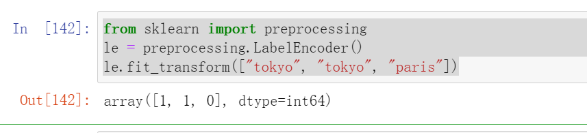
例如:
from sklearn import preprocessing
le = preprocessing.LabelEncoder()
le.fit_transform(["tokyo", "tokyo", "paris"])
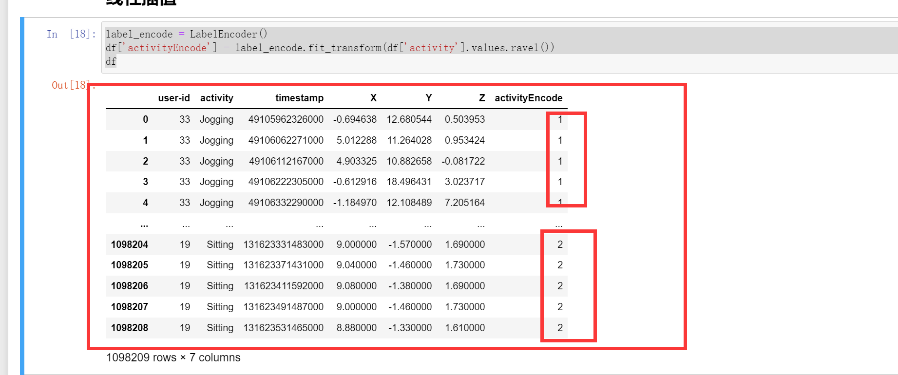
label_encode = LabelEncoder()
df['activityEncode'] = label_encode.fit_transform(df['activity'])
df
线性插值
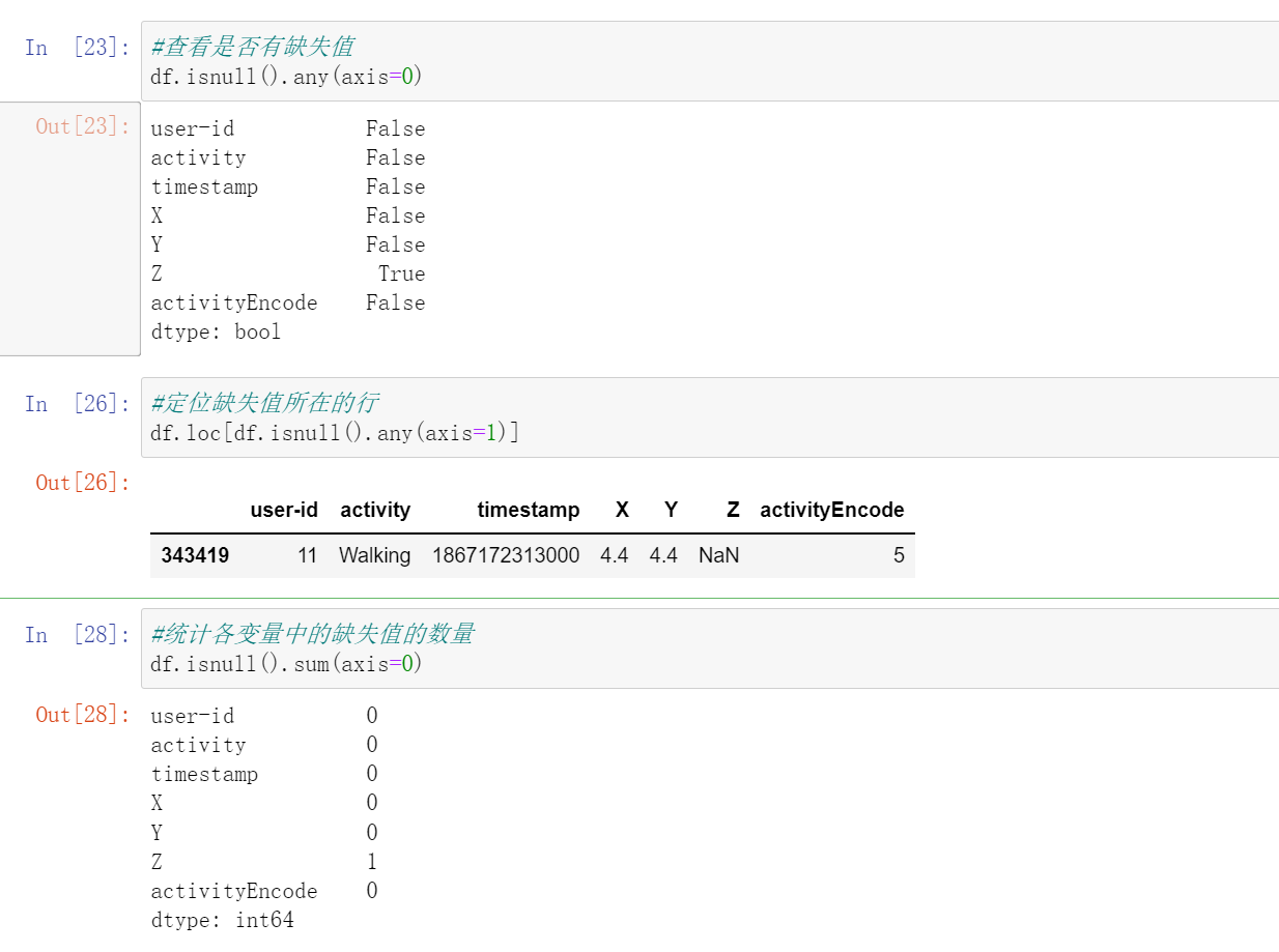
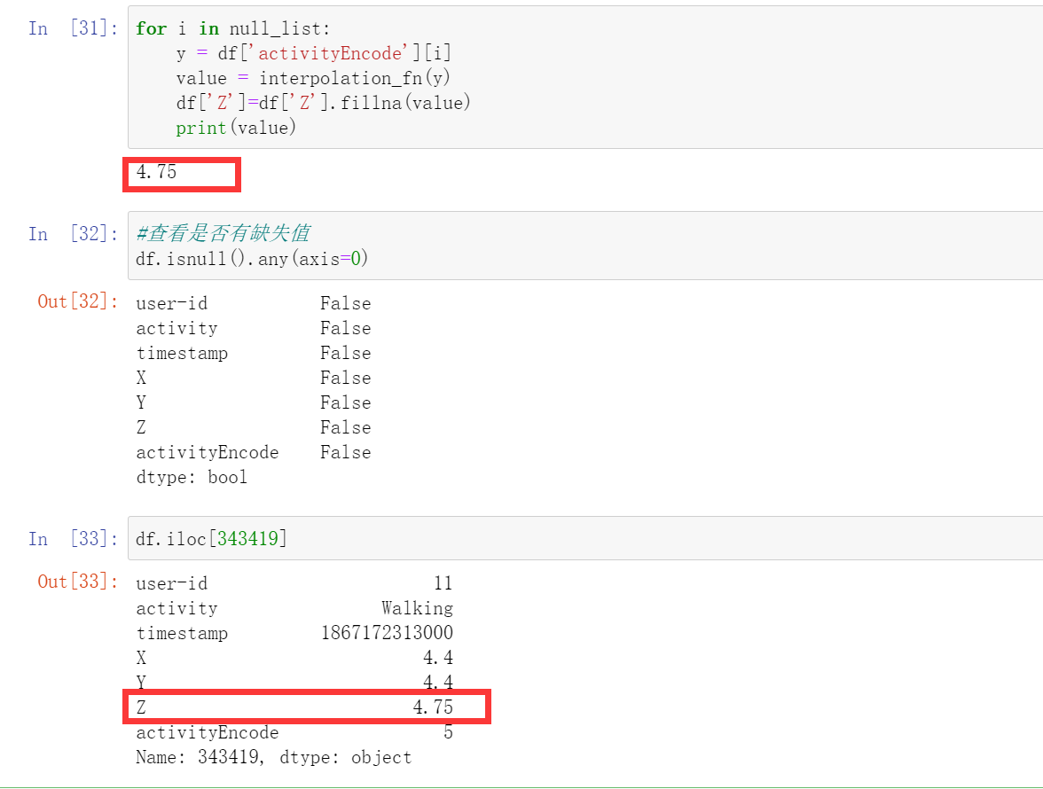
首先查看是否有缺失值
利用线性插值可以避免采集过程中出现NaN的数据丢失的问题。它将通过插值法填充缺失的值。虽然在这个数据集中只有一个NaN值。
查看是否有缺失值:
#查看是否有缺失值
df.isnull().any(axis=0)
#定位缺失值所在的行
df.loc[df.isnull().any(axis=1)]
#统计各变量中的缺失值的数量
df.isnull().sum(axis=0)
线性插值,或者我们可以直接把这一行的数据删除掉,因为我我们的数据很多
interpolation_fn = interp1d(df['activityEncode'] ,df['Z'], kind='linear')
null_list = df[df['Z'].isnull()].index.tolist()
null_list

for i in null_list:
    y = df['activityEncode'][i]
    value = interpolation_fn(y)
    df['Z']=df['Z'].fillna(value)
    print(value)
数据分割
这里我们可以用sklearn进行分割,或者我们可以直接根据user-id进行分割。
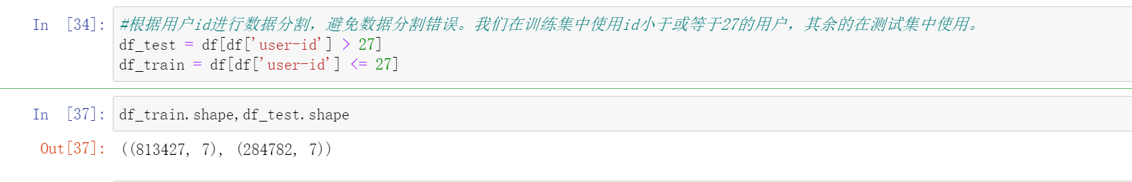
#根据用户id进行数据分割,避免数据分割错误。我们在训练集中使用id小于或等于27的用户,其余的在测试集中使用。
df_test = df[df['user-id'] > 27]
df_train = df[df['user-id'] <= 27]
df_train.shape,df_test.shape
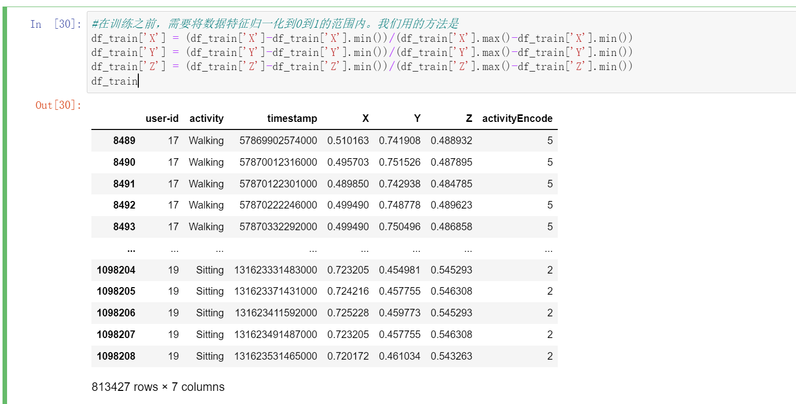
数据无量纲化,归一化
我们这里用到的是:
\(X_i\)=\(\frac{X_i-X_{min}}{X_{max}-X_{min}}\)
#在训练之前,需要将数据特征归一化到0到1的范围内。我们用的方法是
df_train['X'] = (df_train['X']-df_train['X'].min())/(df_train['X'].max()-df_train['X'].min())
df_train['Y'] = (df_train['Y']-df_train['Y'].min())/(df_train['Y'].max()-df_train['Y'].min())
df_train['Z'] = (df_train['Z']-df_train['Z'].min())/(df_train['Z'].max()-df_train['Z'].min())
df_train
时间序列分割
先说说我自己的理解,首先我们需要用到的数据是'X','Y','Z'和'activityEncode'这四个数据。然后我们training的肯定是'X','Y','Z'上的数据。我们预测行为的时候不是一个时刻的行为,而是一段时间序列的行为。也就是根据一段序列(比如说3秒或者5个数据点)的'X','Y','Z'数据来预测这个一段序列的行为,所以我们需要进行时间序列分割。然后我们每个序列中的标签就是这个一段序列中的行为的众数。也就是这个一段序列中最多的一个行为,就作为这一段序列的行为。
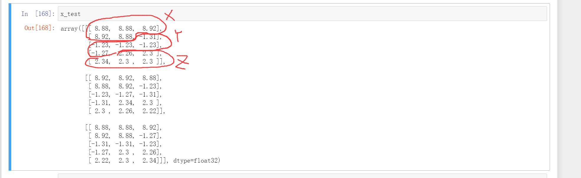
这个我们分割完是一个[b,time_steps,n_features],其中这个n_features是'X','Y','Z'三个特征。
这里我们在处理的时候用到了滑动窗口的知识。我们这里在划分每个序列的时侯,这个序列和下一个序列会有重复的,就像下面一样。
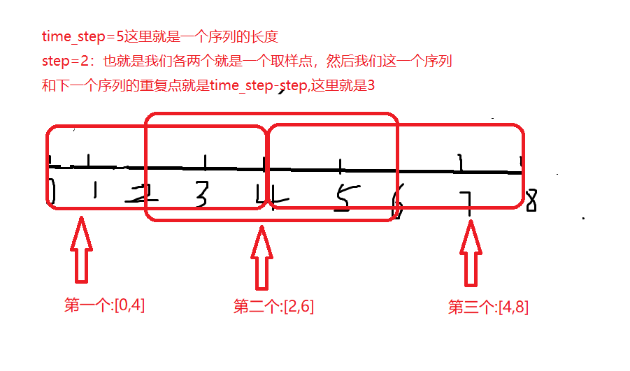
我们最重要得到的是[b,time_steps,n_features],这个b是一共有多少个。time_steps是处理好的序列中有多少个时间点,n_features是一共有多少个特征。
我们还需要设置一个值就是step,就是我们每隔几个点来取一个值,也就是上一个和下一个重复的有time_steps-step个时间点。然后这一段序列中的行为就用这一段的行为标签中的众数来代替。
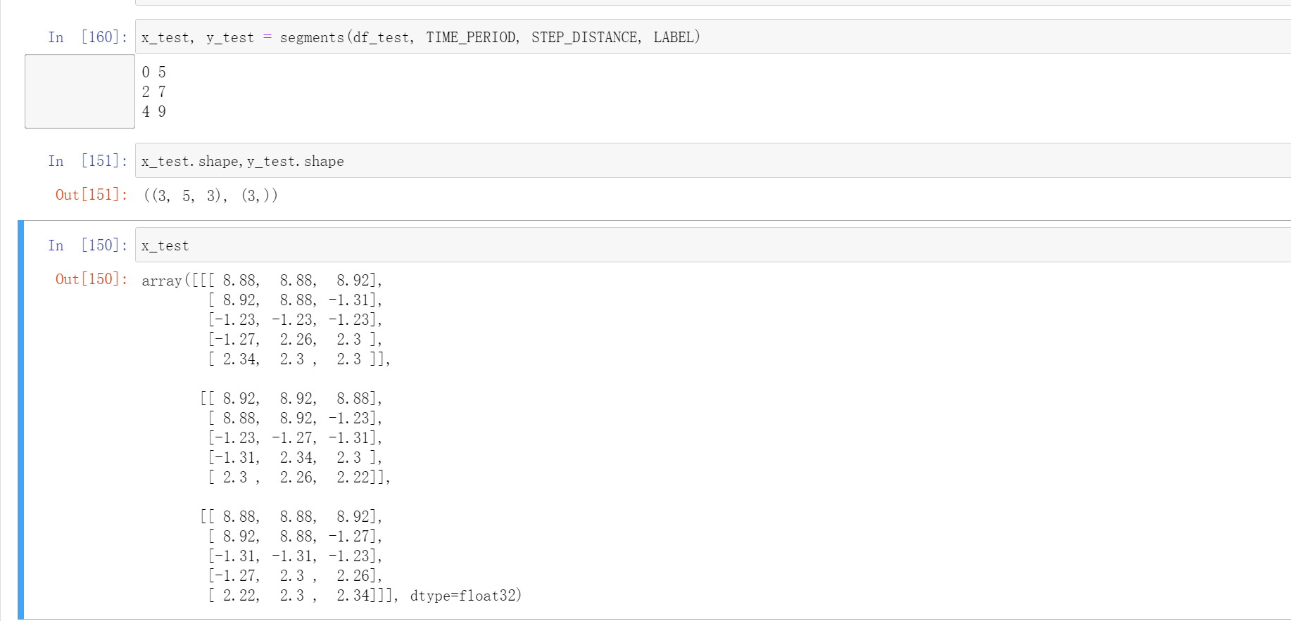
比如我们用time_steps=5,step=2。我们总的数据有9个[0,9)。
第一个就是[0,5):0,1,2,3,4
第二个就是[2,7): 2, 3, 4, 5, 6
第三个就是[4,9): 4, 5, 6, 7, 8
测试:
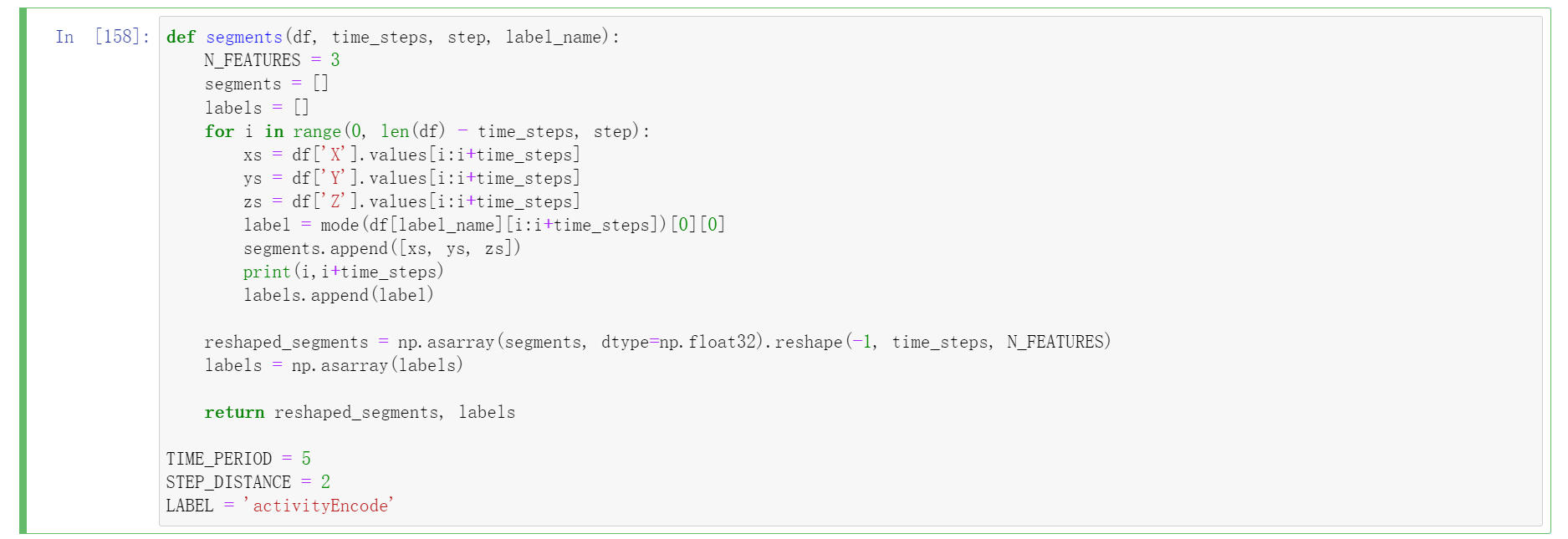
#这里我们设置time_steps=5,step=2,测试一下
def segments(df, time_steps, step, label_name):
    N_FEATURES = 3
    segments = []
    labels = []
    for i in range(0, len(df) - time_steps, step):
        xs = df['X'].values[i:i+time_steps]
        ys = df['Y'].values[i:i+time_steps]
        zs = df['Z'].values[i:i+time_steps]
        label = mode(df[label_name][i:i+time_steps])[0][0]
        segments.append([xs, ys, zs])
        print(i,i+time_steps)
        labels.append(label)

    reshaped_segments = np.asarray(segments, dtype=np.float32).reshape(-1, time_steps, N_FEATURES)
    labels = np.asarray(labels)

    return reshaped_segments, labels

TIME_PERIOD = 5
STEP_DISTANCE = 2
LABEL = 'activityEncode'
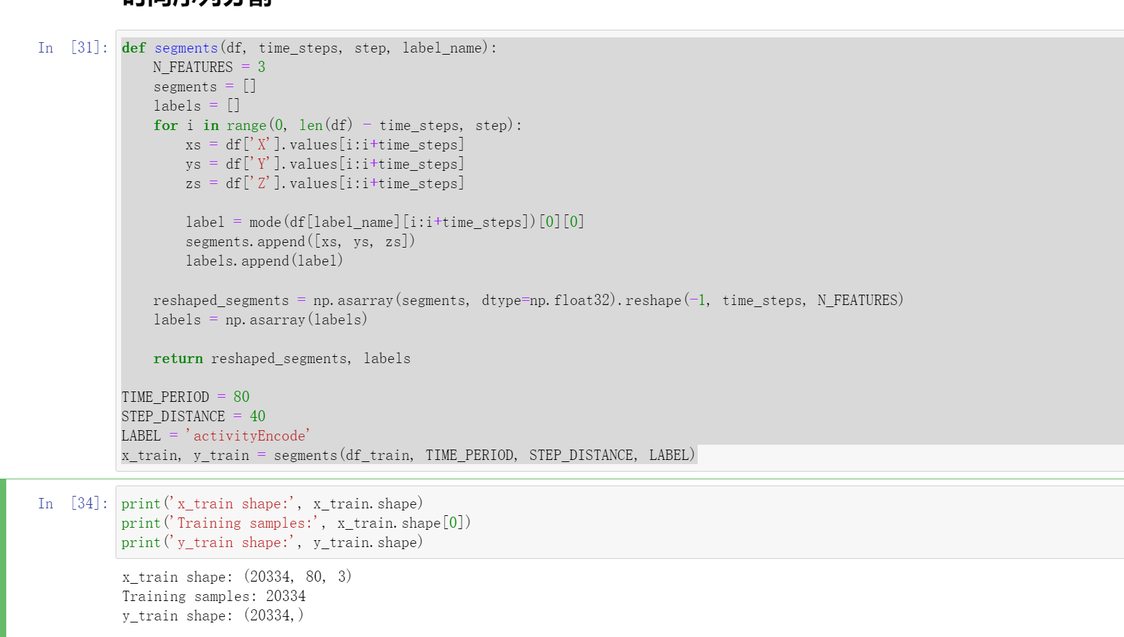
然后我们的处理就是:
def segments(df, time_steps, step, label_name):
    N_FEATURES = 3
    segments = []
    labels = []
    for i in range(0, len(df) - time_steps, step):
        xs = df['X'].values[i:i+time_steps]
        ys = df['Y'].values[i:i+time_steps]
        zs = df['Z'].values[i:i+time_steps]

        label = mode(df[label_name][i:i+time_steps])[0][0]
        segments.append([xs, ys, zs])
        labels.append(label)

    reshaped_segments = np.asarray(segments, dtype=np.float32).reshape(-1, time_steps, N_FEATURES)
    labels = np.asarray(labels)

    return reshaped_segments, labels

TIME_PERIOD = 80
STEP_DISTANCE = 40
LABEL = 'activityEncode'
x_train, y_train = segments(df_train, TIME_PERIOD, STEP_DISTANCE, LABEL)
print('x_train shape:', x_train.shape)
print('Training samples:', x_train.shape[0])
print('y_train shape:', y_train.shape)
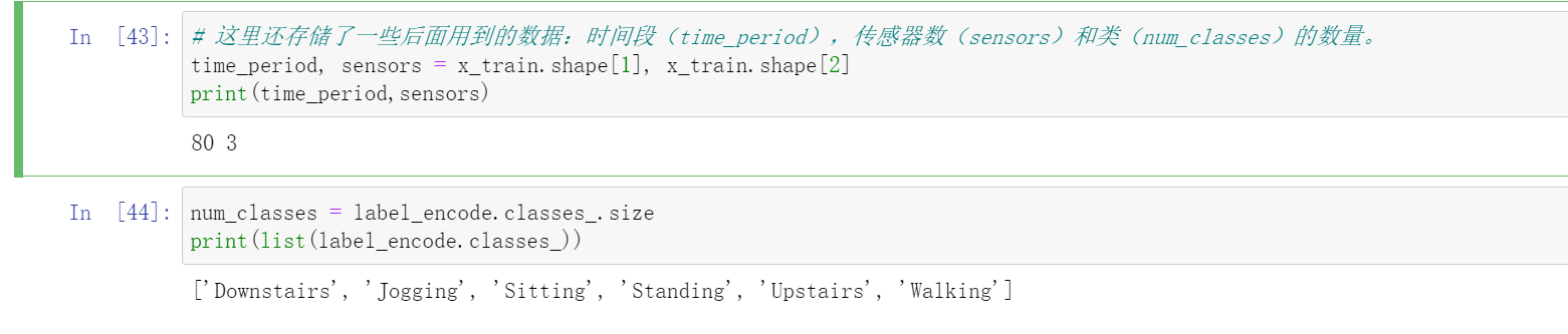
这里还存储了一些后面用到的数据:时间段(time_period),传感器数(sensors)和类(num_classes)的数量。
这里的time_period是80,传感器个数就是3(X,Y,Z),类的数量就是:['Downstairs', 'Jogging', 'Sitting', 'Standing', 'Upstairs', 'Walking']。
# 这里还存储了一些后面用到的数据:时间段(time_period),传感器数(sensors)和类(num_classes)的数量。
time_period, sensors = x_train.shape[1], x_train.shape[2]
print(time_period,sensors)
num_classes = label_encode.classes_.size
print(list(label_encode.classes_))
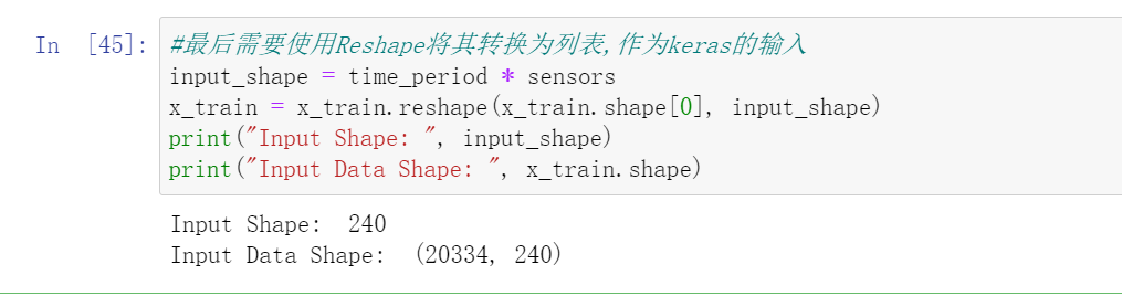
最后需要使用Reshape将其转换为列表,作为keras的输入
#最后需要使用Reshape将其转换为列表,作为keras的输入
input_shape = time_period * sensors
x_train = x_train.reshape(x_train.shape[0], input_shape)
print("Input Shape: ", input_shape)
print("Input Data Shape: ", x_train.shape)
最后需要将所有数据转换为float32。
# 最后需要将所有数据转换为float32。
x_train = x_train.astype('float32')
y_train = y_train.astype('float32')
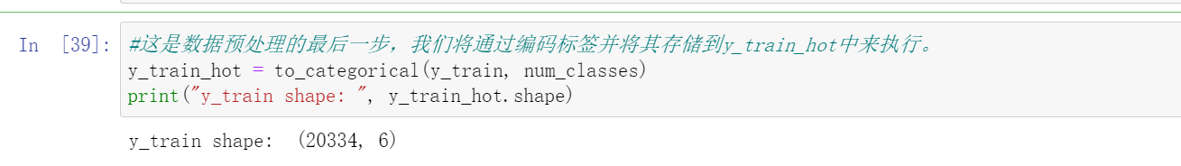
独热编码
#这是数据预处理的最后一步,我们将通过编码标签并将其存储到y_train_hot中来执行。
y_train_hot = to_categorical(y_train, num_classes)
print("y_train shape: ", y_train_hot.shape)
模型预测
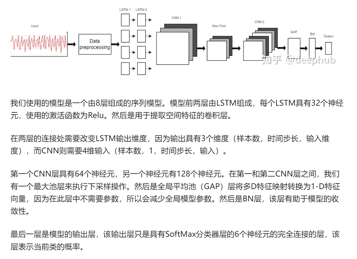
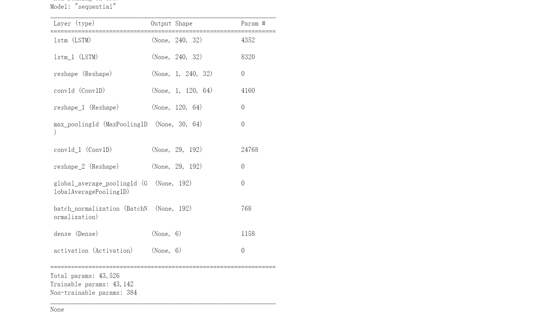
model = Sequential()
model.add(LSTM(32, return_sequences=True, input_shape=(input_shape,1), activation='relu'))
model.add(LSTM(32,return_sequences=True, activation='relu'))
model.add(Reshape((1, 240, 32)))
model.add(Conv1D(filters=64,kernel_size=2, activation='relu', strides=2))
model.add(Reshape((120, 64)))
model.add(MaxPool1D(pool_size=4, padding='same'))
model.add(Conv1D(filters=192, kernel_size=2, activation='relu', strides=1))
model.add(Reshape((29, 192)))
model.add(GlobalAveragePooling1D())
model.add(BatchNormalization(epsilon=1e-06))
model.add(Dense(6))
model.add(Activation('softmax'))

print(model.summary())
training
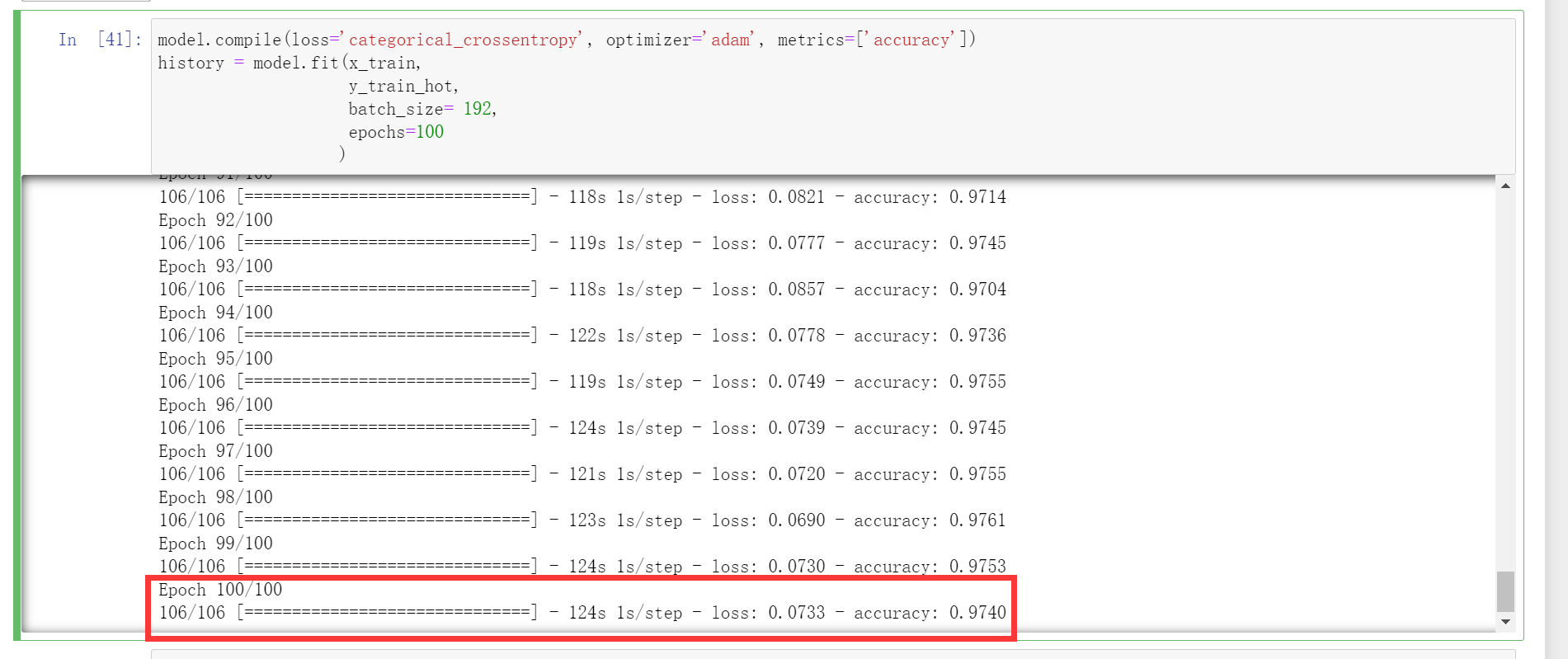
model.compile(loss='categorical_crossentropy', optimizer='adam', metrics=['accuracy'])
history = model.fit(x_train,
                    y_train_hot,
                    batch_size= 192,
                    epochs=100
                   )
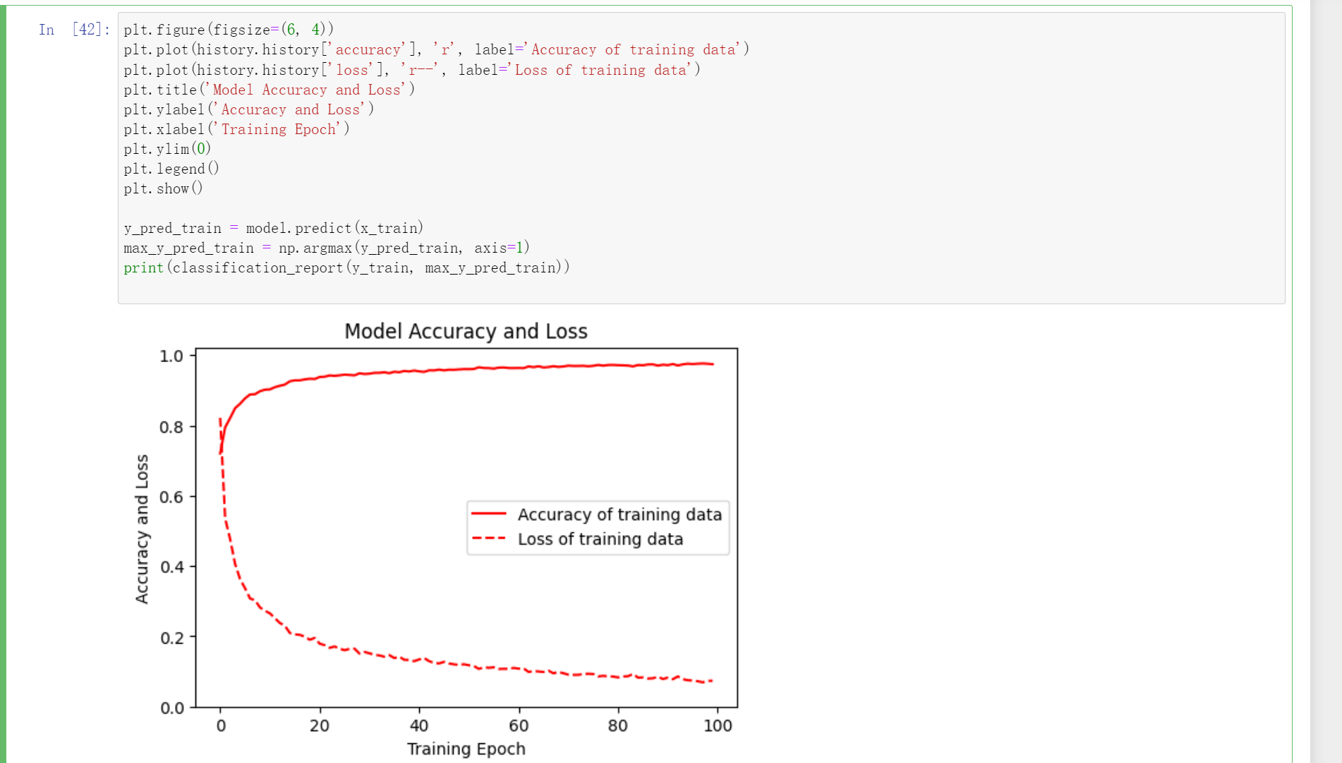
作图
plt.figure(figsize=(6, 4))
plt.plot(history.history['accuracy'], 'r', label='Accuracy of training data')
plt.plot(history.history['loss'], 'r--', label='Loss of training data')
plt.title('Model Accuracy and Loss')
plt.ylabel('Accuracy and Loss')
plt.xlabel('Training Epoch')
plt.ylim(0)
plt.legend()
plt.show()
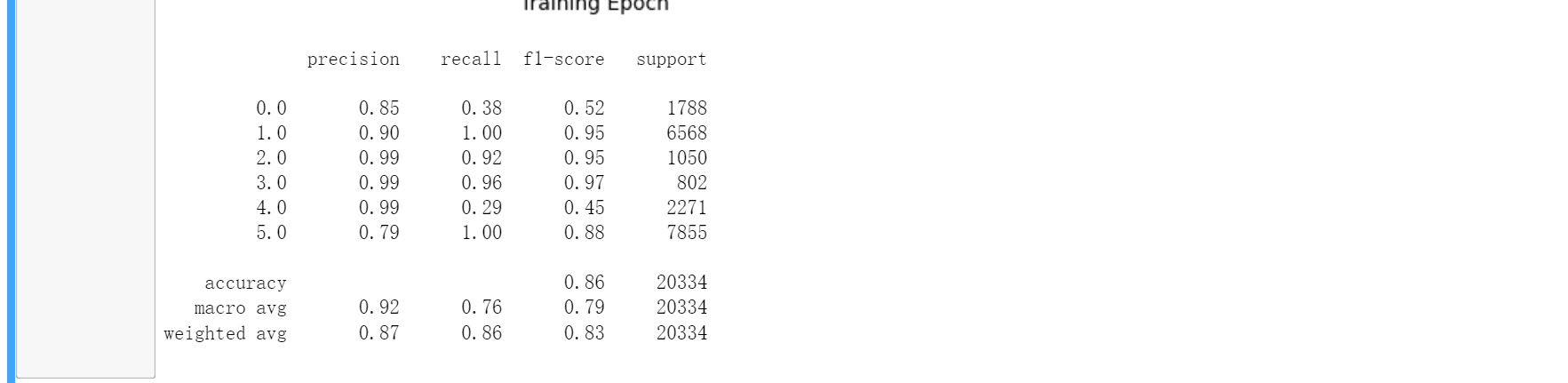
y_pred_train = model.predict(x_train)
max_y_pred_train = np.argmax(y_pred_train, axis=1)
print(classification_report(y_train, max_y_pred_train))