本文基于Jupyter Notebook编写,旨在对零售超市数据集进行探索性分析。
数据集来源数据来源:https://www.kaggle.com/datasets/roopacalistus/superstore
数据及含义
该数据集包含在美国不同地区拥有多家商店的连锁超市的不同商店的销售详细信息。
数据包含如下列(供参考,进一步请查看源数据):
Ship Mode:运输模式
Segment:划分
Country:国家
City:城市
State:州
Postal code:邮政编码
Region:地区
Category:类目
Sub-category:子类
Sales:销售额
Quantity:数量
Discount:折扣
Profit:利润
导入库和数据
import pandas as pd
import numpy as np
import seaborn as sns
import matplotlib.pyplot as plt
import os
# jupter魔法函数,设置可视化页内显示
%matplotlib inline
# 正常显示中文和负号
plt.rcParams['font.sans-serif'] = ['SimHei']
plt.rcParams['axes.unicode_minus'] = False
# 画图的样式风格设置为:ggplot
plt.style.use('ggplot')
# 导入数据集
# 设定默认工作路径
os.chdir(r'F:\py_jupyter_notebook\data')

df = pd.read_csv('SampleSuperstore.csv')
# 查看数据集前五行
df.head()
| Ship Mode | Segment | Country | City | State | Postal Code | Region | Category | Sub-Category | Sales | Quantity | Discount | Profit | |
|---|---|---|---|---|---|---|---|---|---|---|---|---|---|
| 0 | Second Class | Consumer | United States | Henderson | Kentucky | 42420 | South | Furniture | Bookcases | 261.9600 | 2 | 0.00 | 41.9136 |
| 1 | Second Class | Consumer | United States | Henderson | Kentucky | 42420 | South | Furniture | Chairs | 731.9400 | 3 | 0.00 | 219.5820 |
| 2 | Second Class | Corporate | United States | Los Angeles | California | 90036 | West | Office Supplies | Labels | 14.6200 | 2 | 0.00 | 6.8714 |
| 3 | Standard Class | Consumer | United States | Fort Lauderdale | Florida | 33311 | South | Furniture | Tables | 957.5775 | 5 | 0.45 | -383.0310 |
| 4 | Standard Class | Consumer | United States | Fort Lauderdale | Florida | 33311 | South | Office Supplies | Storage | 22.3680 | 2 | 0.20 | 2.5164 |
通过数据的前5行可以初步了解数据集包含的信息。
# 查看数据基本信息
df.info()
<class 'pandas.core.frame.DataFrame'>
RangeIndex: 9994 entries, 0 to 9993
Data columns (total 13 columns):
 #   Column        Non-Null Count  Dtype
---  ------        --------------  -----
 0   Ship Mode     9994 non-null   object
 1   Segment       9994 non-null   object
 2   Country       9994 non-null   object
 3   City          9994 non-null   object
 4   State         9994 non-null   object
 5   Postal Code   9994 non-null   int64
 6   Region        9994 non-null   object
 7   Category      9994 non-null   object
 8   Sub-Category  9994 non-null   object
 9   Sales         9994 non-null   float64
 10  Quantity      9994 non-null   int64
 11  Discount      9994 non-null   float64
 12  Profit        9994 non-null   float64
dtypes: float64(3), int64(2), object(8)
memory usage: 1015.1+ KB
可以看到数据集中没有空值,接下来对重复值进行验证并去重。将去重之后的数据集保存在df1中。
df.duplicated()
0       False
1       False
2       False
3       False
4       False
        ...
9989    False
9990    False
9991    False
9992    False
9993    False
Length: 9994, dtype: bool
df.duplicated().sum()
17
df1 = df.drop_duplicates()
# df.drop_duplicates(inplace = True) 这样是做原数据框上的修改并替换
df1.duplicated().sum()
0
可以看到重复值为0,即去重完成。
df1.info()
<class 'pandas.core.frame.DataFrame'>
Int64Index: 9977 entries, 0 to 9993
Data columns (total 13 columns):
 #   Column        Non-Null Count  Dtype
---  ------        --------------  -----
 0   Ship Mode     9977 non-null   object
 1   Segment       9977 non-null   object
 2   Country       9977 non-null   object
 3   City          9977 non-null   object
 4   State         9977 non-null   object
 5   Postal Code   9977 non-null   int64
 6   Region        9977 non-null   object
 7   Category      9977 non-null   object
 8   Sub-Category  9977 non-null   object
 9   Sales         9977 non-null   float64
 10  Quantity      9977 non-null   int64
 11  Discount      9977 non-null   float64
 12  Profit        9977 non-null   float64
dtypes: float64(3), int64(2), object(8)
memory usage: 1.1+ MB
得到有效数据9977条。其中邮政编码这一列对分析工作并无作用,将其从数据框中去掉,并保存在数据框data中。
data = df1.drop(["Postal Code"], axis=1)
data.info()
<class 'pandas.core.frame.DataFrame'>
Int64Index: 9977 entries, 0 to 9993
Data columns (total 12 columns):
 #   Column        Non-Null Count  Dtype
---  ------        --------------  -----
 0   Ship Mode     9977 non-null   object
 1   Segment       9977 non-null   object
 2   Country       9977 non-null   object
 3   City          9977 non-null   object
 4   State         9977 non-null   object
 5   Region        9977 non-null   object
 6   Category      9977 non-null   object
 7   Sub-Category  9977 non-null   object
 8   Sales         9977 non-null   float64
 9   Quantity      9977 non-null   int64
 10  Discount      9977 non-null   float64
 11  Profit        9977 non-null   float64
dtypes: float64(3), int64(1), object(8)
memory usage: 1013.3+ KB
数据分析
为了探究变量之间的相关性,计算数字类型的数据(Sales、Quantity、Discount、Profit)的相关系数。
data.corr(method = 'pearson',numeric_only = 'True')
# numeric_only,仅数字,布尔型,默认False。如果为True,则仅适用于数字列
| Sales | Quantity | Discount | Profit | |
|---|---|---|---|---|
| Sales | 1.000000 | 0.200722 | -0.028311 | 0.479067 |
| Quantity | 0.200722 | 1.000000 | 0.008678 | 0.066211 |
| Discount | -0.028311 | 0.008678 | 1.000000 | -0.219662 |
| Profit | 0.479067 | 0.066211 | -0.219662 | 1.000000 |
sns.heatmap(data.corr(numeric_only = 'True'), annot=True,fmt = 'f')
# heatmap中的参数annot为True时,为每个单元格写入数据值。如果数组具有与数据相同的形状,则使用它来注释热力图而不是原始数据。参数fmt是指添加注释时要使用的字符串格式代码:d 整数 f 浮点数 s 字符串
<Axes: >
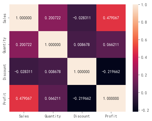
对于相关系数作热力图以更直观的看到相关性大小。其中,销量与利润呈显著正相关,折扣与利润呈负相关。
data["Ship Mode"].value_counts()
Standard Class    5955
Second Class      1943
First Class       1537
Same Day           542
Name: Ship Mode, dtype: int64
sns.countplot(x= data['Ship Mode'])
<Axes: xlabel='Ship Mode', ylabel='count'>
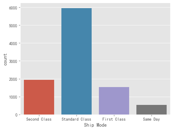
对于运输模式下的各个细分属性进行统计,并作条形统计图,得到标准运输的订单最多。
sns.countplot(x= data['Segment'])
<Axes: xlabel='Segment', ylabel='count'>

同样的,对于用户划分下的各个细分属性进行统计,并作条形统计图,可以看到个体消费者最多。
data["Category"].value_counts()
Office Supplies    6012
Furniture          2118
Technology         1847
Name: Category, dtype: int64
sns.countplot(x= data['Category'])
<Axes: xlabel='Category', ylabel='count'>

可以看到,购买商品的类目中,办公用品最多。
data["Sub-Category"].value_counts()
Binders        1522
Paper          1359
Furnishings     956
Phones          889
Storage         846
Art             795
Accessories     775
Chairs          615
Appliances      466
Labels          363
Tables          319
Envelopes       254
Bookcases       228
Fasteners       217
Supplies        190
Machines        115
Copiers          68
Name: Sub-Category, dtype: int64
plt.figure(figsize=(10,10))
plt.pie(data["Sub-Category"].value_counts(), labels= data["Sub-Category"].value_counts().index, autopct ="%2f")
plt.show()
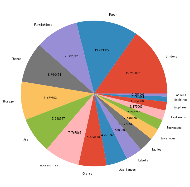
将子分类做饼图,可以看到纸和装订机占比最多,两者合计占比约30%.
st_profit=data.groupby(["State"])["Profit"].sum().nlargest(20)
# nlargest()的第一个参数就是截取的行数。第二个参数就是依据的列名。
# nlargest()的优点就是能一次看到最大的几行,而且不需要排序。缺点就是只能看到最大的,看不到最小的。
st_profit
State
California       76330.7891
New York         74015.4622
Washington       33368.2375
Michigan         24428.0903
Virginia         18597.9504
Indiana          18382.9363
Georgia          16250.0433
Kentucky         11199.6966
Minnesota        10823.1874
Delaware          9977.3748
New Jersey        9772.9138
Wisconsin         8401.8004
Rhode Island      7285.6293
Maryland          7031.1788
Massachusetts     6785.5016
Missouri          6436.2105
Alabama           5786.8253
Oklahoma          4853.9560
Arkansas          4008.6871
Connecticut       3511.4918
Name: Profit, dtype: float64
plt.figure(figsize=(15,8))
st_profit.plot.bar()
<Axes: xlabel='State'>
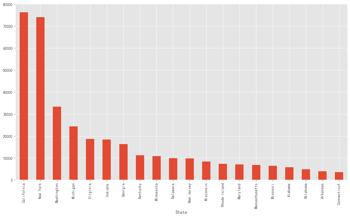
找到利润最多的前20个州,并按从大到小的顺序绘制条形统计图,加利福利亚和纽约的利润远高出其他州。
sns.lineplot(data=data, x="Discount", y= "Profit")
# Discount和Profit都是一组数据,在拟合时产生的阴影由此而来。
<Axes: xlabel='Discount', ylabel='Profit'>
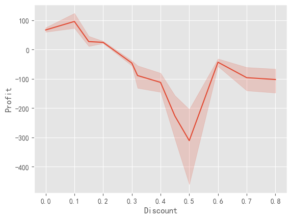
对于折扣和利润的关系进一步作折线图,看到当折扣为0.5时,利润取最小值。
data.plot(kind="scatter",x="Sales",y="Profit", c="Discount", colormap="Set1",figsize=(10,10))
<Axes: xlabel='Sales', ylabel='Profit'>
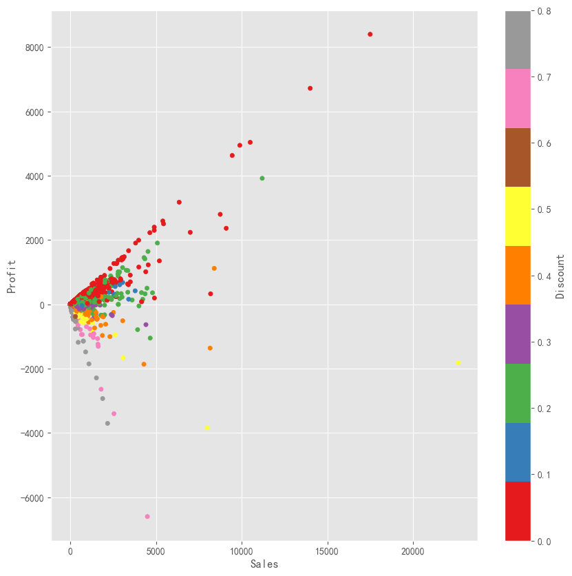
在这个散点图中,我们可以清楚地看到,更多的销售额并不意味着更多的利润,它也取决于折扣。当销售额高而折扣低时,利润率更高。
data1= data.groupby("State")[["Sales","Profit"]].sum().sort_values(by="Sales", ascending=False)
data1[:].plot.bar(color = ["Green","Red"], figsize=(20,12))
plt.title("Profit-Loss and Sales across States")
plt.show()
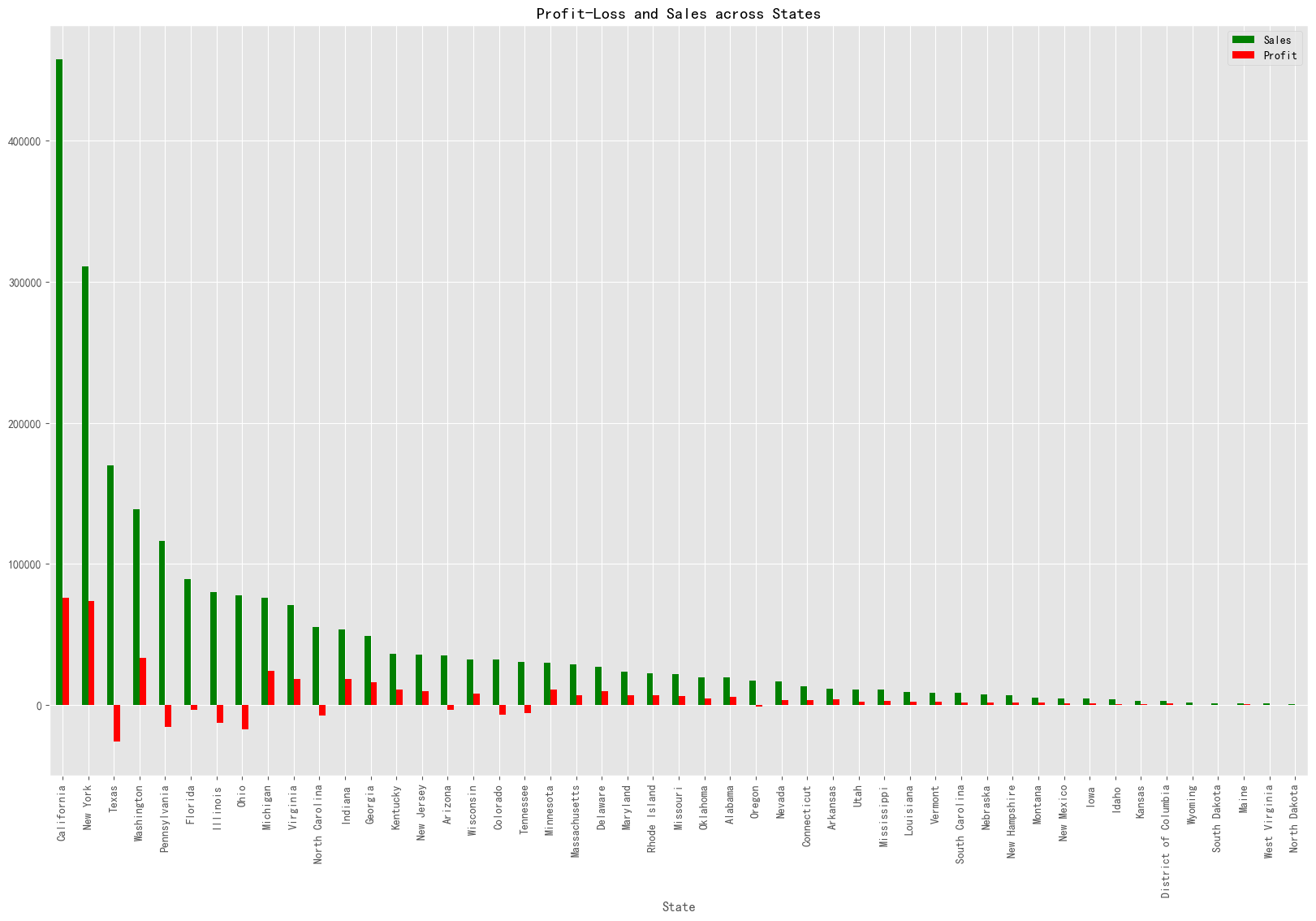
与其他州相比,加利福尼亚州和纽约州产生更多的利润。
data1= data.groupby("Region")[["Sales","Profit"]].sum().sort_values(by="Sales", ascending=False)
data1[:].plot.bar(color = ["Blue","Red"], figsize=(10,7))
plt.title("Profit-Loss and Sales across Region")
plt.show()
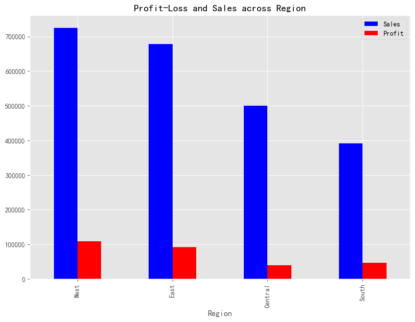
可以得到以下结论:
西部地区利润最高。 与其他地方相比,加利福尼亚,纽约和华盛顿产生的销售额最多。 中部地区产生的利润最低。 德克萨斯州,宾夕法尼亚州,佛罗里达州,伊利诺伊州,俄亥俄州和其他一些州正在产生高额销售的损失。因此,我们需要对它们给予一些关注。 因此,我们必须在加利福尼亚和纽约做更多的工作。通过减少德克萨斯州、佛罗里达州、俄亥俄州等州的销售额来增加这些州的销售额。通过降低中部地区的贴现率,我们可以增加利润。最后,我们应该增加办公用品类别的销售,因为它们的贡献更大。