一、选题的背景
近年来,随着全球经济的发展,水果消费市场规模不断扩大,水果种类也日益丰富,水果检测与识别技术在农业生产、仓储物流、超市零售等领域具有重要的应用价值,传统的水果检测与识别方法。主要依赖于人工识别,这种方法在一定程度上受到人力成本、识别效率和准确性等方面的限制。因此,开发一种高效准确的自动化水果检测与识别系统具有重要的研究意义和实际价值。
二、机器学习案例设计方案
1.本选题采用的机器学习案例来源
数据集来源:Kaggle 网址:https://www.kaggle.com/
2.采用的机器学习框架描述
通过神经网络模型的构建过程来实现目的
3.涉及到技术难点与解决思路
难点:神经网络那一块比较难
解决思路:通过网络视频来解决难点
三、机器学习的实现步骤
1.数据集下载

2.导入所需要的库
#导入需要使用的库
import matplotlib.pyplot as plt
import numpy as np
import pandas as pd
from pathlib import Path
import os
import PIL
import tensorflow as tf
from tensorflow import keras
from tensorflow.keras import layers
from tensorflow.keras.models import Sequential
3.获取训练集、测试集、验证集的文件路径
TEST_DIR = r'C:\Users\chy\jzj\test'
TRAIN_DIR =r'C:\Users\chy\jzj\train'
VALID_DIR =r'C:\Users\chy\jzj\validation'
4.加载数据集及更改图片属性
train_generator = tf.keras.preprocessing.image.ImageDataGenerator(
    preprocessing_function=tf.keras.applications.mobilenet_v2.preprocess_input
)

test_generator = tf.keras.preprocessing.image.ImageDataGenerator(
    preprocessing_function=tf.keras.applications.mobilenet_v2.preprocess_input
)

#从文件夹中加载训练集
train_images = train_generator.flow_from_dataframe(
    dataframe=train_df,
    x_col='Filepath',
    y_col='Label',
    target_size=(224, 224),
    color_mode='rgb',
    class_mode='categorical',
    batch_size=32,
    shuffle=True,
    seed=0,
    rotation_range=30,
    zoom_range=0.15,
    width_shift_range=0.2,
    height_shift_range=0.2,
    shear_range=0.15,
    horizontal_flip=True,
    fill_mode="nearest"
)

#从文件夹中加载训练集
val_images = train_generator.flow_from_dataframe(
    dataframe=val_df,
    x_col='Filepath',
    y_col='Label',
    target_size=(224, 224),
    color_mode='rgb',
    class_mode='categorical',
    batch_size=32,
    shuffle=True,
    seed=0,
    rotation_range=30,
    zoom_range=0.15,
    width_shift_range=0.2,
    height_shift_range=0.2,
    shear_range=0.15,
    horizontal_flip=True,
    fill_mode="nearest"
)

#从文件夹中加载训练集
test_images = test_generator.flow_from_dataframe(
    dataframe=test_df,
    x_col='Filepath',
    y_col='Label',
    target_size=(224, 224),
    color_mode='rgb',
    class_mode='categorical',
    batch_size=32,
    shuffle=False
)

train_ds = tf.keras.preprocessing.image_dataset_from_directory(TRAIN_DIR,
                                                               seed=2509,
                                                               image_size=(img_height, img_width),
                                                               batch_size=batch_size)

valid_ds = tf.keras.preprocessing.image_dataset_from_directory(VALID_DIR,
                                                               seed=2509,
                                                               image_size=(img_height, img_width),
                                                               shuffle=False,
                                                               batch_size=batch_size)

test_ds = tf.keras.preprocessing.image_dataset_from_directory(TEST_DIR,
                                                              seed=2509,
                                                              image_size=(img_height, img_width),
                                                              shuffle=False,
                                                              batch_size=batch_size)

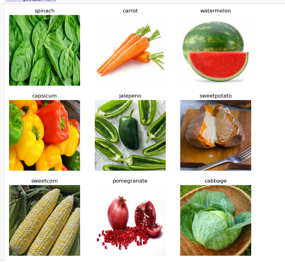
5.查看图片
import matplotlib.pyplot as plt

#从训练集数据集中取出一个数据
plt.figure(figsize=(10, 10))
for images, labels in train_ds.take(1):
    for i in range(9):
        ax = plt.subplot(3, 3, i + 1)
        plt.imshow(images[i].numpy().astype("uint8"))
        plt.title(class_names[labels[i]])
        plt.axis("off")
6.获取分类名称
class_names = train_ds.class_names
print(class_names)

7.神经网络训练过程
#定义模型结构
inputs = tf.keras.Input(shape=(224,224,3))
x = tf.keras.layers.experimental.preprocessing.Rescaling(1./255)(inputs)
x = data_augmentation(x)
x = base_model(x,training=False)
x = tf.keras.layers.GlobalAveragePooling2D()(x)#对卷积神经网络的输出进行全局平均池化操作
x = tf.keras.layers.Flatten()(x)
#包含1024个神经元的全连接层
x = tf.keras.layers.Dense(1024,activation='relu')(x)
#包含512个神经元的全连接层
x = tf.keras.layers.Dense(512,activation='relu')(x)
#添加输出层
x = tf.keras.layers.Dense(len(class_names),activation='softmax')(x)
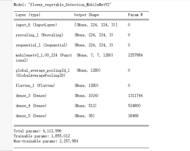
8.输出模型信息
model.summary()
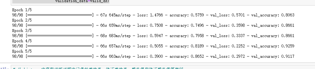
9.第一次模型训练
history = model.fit(x=train_ds,
                    epochs= initial_epochs,
                    validation_data=valid_ds)
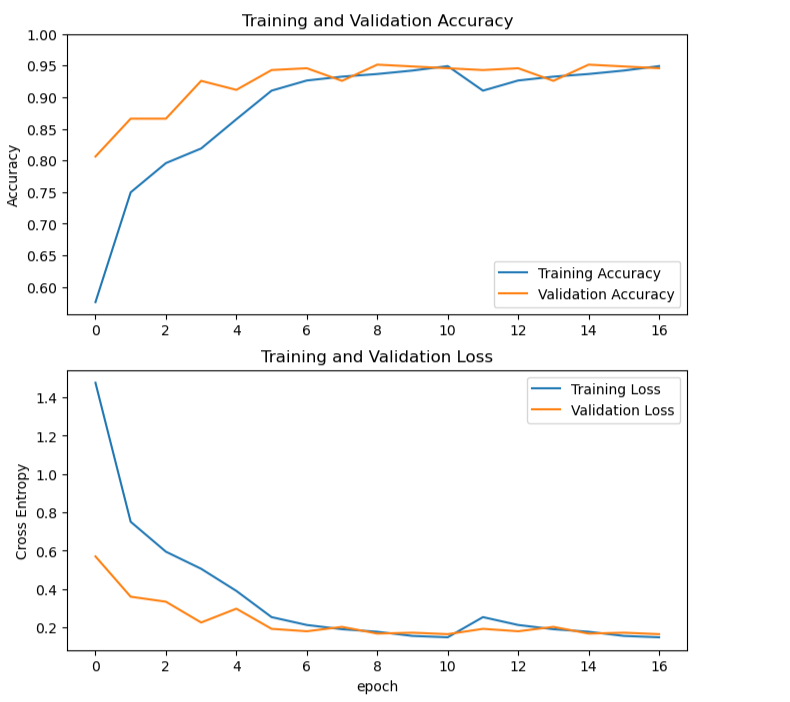
根据训练结果,输出准确率、验证准确率、损失值和验证损失值等指标的图形
acc = history.history['accuracy']
val_acc = history.history['val_accuracy']

loss = history.history['loss']
val_loss = history.history['val_loss']

# 使用 Matplotlib 库将训练准确率(Training Accuracy)、验证准确率(Validation Accuracy)、训练损失值(Training Loss)和验证损失值(Validation Loss)分别绘制成两张子图,展示训练和验证的变化趋势
plt.figure(figsize=(8, 8))
plt.subplot(2, 1, 1)
plt.plot(acc, label='Training Accuracy')
plt.plot(val_acc, label='Validation Accuracy')
plt.legend(loc='lower right')
plt.ylabel('Accuracy')
plt.ylim([min(plt.ylim()),1])
plt.title('Training and Validation Accuracy')

plt.subplot(2, 1, 2)
plt.plot(loss, label='Training Loss')
plt.plot(val_loss, label='Validation Loss')
plt.legend(loc='upper right')
plt.ylabel('Cross Entropy')
plt.title('Training and Validation Loss')
plt.xlabel('epoch')
plt.show()
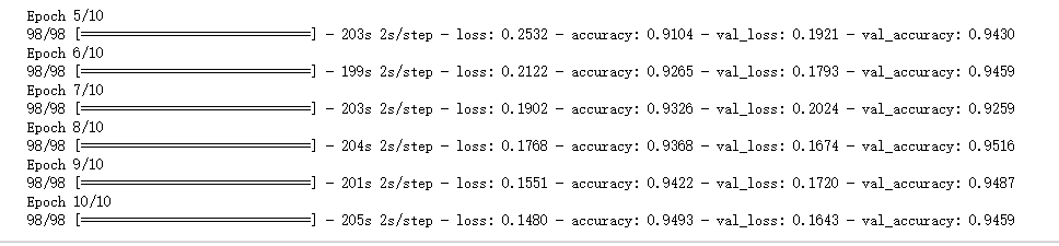
10.第二次模型训练(微调过后)
fine_tune_epochs = 5
total_epochs =  initial_epochs + fine_tune_epochs

#对模型进行调整
history_fine = model.fit(train_ds,
                         epochs=total_epochs,
                         initial_epoch=history.epoch[-1],
                         validation_data=valid_ds)
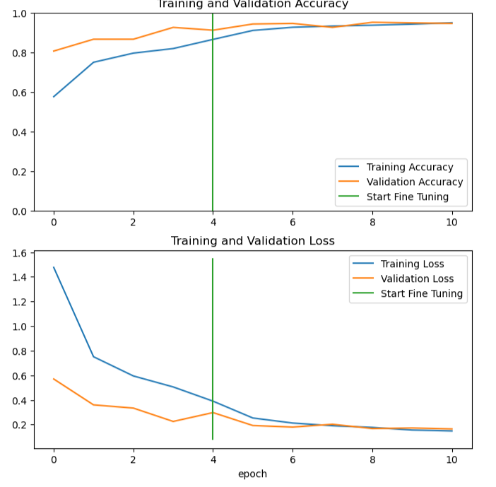
根据第二次训练结果,输出准确率、验证准确率、损失值和验证损失值等指标的图形
# 绘制微调后的模型训练过程中准确率和损失值的变化曲线

plt.figure(figsize=(8, 8))
plt.subplot(2, 1, 1)
plt.plot(acc, label='Training Accuracy')
plt.plot(val_acc, label='Validation Accuracy')
plt.ylim([0.0, 1])
plt.plot([initial_epochs-1,initial_epochs-1],
          plt.ylim(), label='Start Fine Tuning')
plt.legend(loc='lower right')
plt.title('Training and Validation Accuracy')

plt.subplot(2, 1, 2)
plt.plot(loss, label='Training Loss')
plt.plot(val_loss, label='Validation Loss')
plt.plot([initial_epochs-1,initial_epochs-1],
         plt.ylim(), label='Start Fine Tuning')
plt.legend(loc='upper right')
plt.title('Training and Validation Loss')
plt.xlabel('epoch')
plt.show()
四、总结
经过本次学习,我对机器学习及其在果蔬检测和识别中的应用有了更深入的理解和认识。以下是我的学习总结:
1.果蔬的检测和识别是机器学习在农业领域中的应用之一。
2.在果蔬的检测和识别中,我们可以采用神经网络来训练模型,以实现对不同种类的水果和蔬菜进行有效识别。
3.总体来讲,在果蔬检测和识别中应用机器学习可以大幅度提高农业生产效率,同时也为人们提供了更加便捷的果蔬识别和选购方式。
收获:使我的机器学习能力更进一步。
改进:通过这次的编写的程序,察觉的自身还缺乏很多相关知识,以后还需慢慢学习。
五、完整代码
  1 #导入需要使用的库
  2 import matplotlib.pyplot as plt
  3 import numpy as np
  4 import pandas as pd
  5 from pathlib import Path
  6 import os
  7 import PIL
  8 import tensorflow as tf
  9 from tensorflow import keras
 10 from tensorflow.keras import layers
 11 from tensorflow.keras.models import Sequential
 12
 13 # 创建一个包含训练和测试的文件路径列表
 14 train_dir = Path(r'C:\Users\chy\jzj\train')
 15 train_filepaths = list(train_dir.glob(r'**/*.jpg'))
 16
 17 test_dir = Path(r'C:\Users\chy\jzj\test')
 18 test_filepaths = list(test_dir.glob(r'**/*.jpg'))
 19
 20 val_dir = Path(r'C:\Users\chy\jzj\validation')
 21 val_filepaths = list(test_dir.glob(r'**/*.jpg'))
 22
 23 def proc_img(filepath):
 24 #创建一个 DataFrame,其中包含图片的文件路径和标签
 25
 26 # 从文件中提取标签
 27     labels = [str(filepath[i]).split("/")[-1] \
 28               for i in range(len(filepath))]
 29 # 将文件路径和标签转换为 Series 类型,并指定出列名
 30     filepath = pd.Series(filepath, name='Filepath').astype(str)
 31     labels = pd.Series(labels, name='Label')
 32
 33     df = pd.concat([filepath, labels], axis=1)
 34 # 将文件路径和标签拼接成 DataFrame,并随机打乱排序和重置索引
 35     # Shuffle the DataFrame and reset index
 36     df = df.sample(frac=1).reset_index(drop = True)
 37
 38     return df
 39 # 对训练、测试、验证集的文件路径进行处理,得到包含文件路径和标签的 DataFrame
 40 train_df = proc_img(train_filepaths)
 41 test_df = proc_img(test_filepaths)
 42 val_df = proc_img(val_filepaths)
 43
 44 #TRAIN_DIR 表示训练集所在的文件夹路径
 45 #TEST_DIR 表示测试集所在的文件夹路径
 46 #VALID_DIR 表示验证集所在的文件夹路径
 47 TEST_DIR = r'C:\Users\chy\jzj\test'
 48 TRAIN_DIR =r'C:\Users\chy\jzj\train'
 49 VALID_DIR =r'C:\Users\chy\jzj\validation'
 50
 51 #从指定目录 train_ds中加载图片数据集
 52 train_ds = tf.keras.preprocessing.image_dataset_from_directory(TRAIN_DIR,
 53                                                                seed=2509,
 54                                                                image_size=(img_height, img_width),
 55                                                                batch_size=batch_size)
 56
 57 #实例化 ImageDataGenerator 类,进行数据增强操作
 58 train_generator = tf.keras.preprocessing.image.ImageDataGenerator(
 59     preprocessing_function=tf.keras.applications.mobilenet_v2.preprocess_input
 60 )
 61
 62 test_generator = tf.keras.preprocessing.image.ImageDataGenerator(
 63     preprocessing_function=tf.keras.applications.mobilenet_v2.preprocess_input
 64 )
 65
 66 #从文件夹中加载训练集
 67 train_images = train_generator.flow_from_dataframe(
 68     dataframe=train_df,
 69     x_col='Filepath',
 70     y_col='Label',
 71     target_size=(224, 224),
 72     color_mode='rgb',
 73     class_mode='categorical',
 74     batch_size=32,
 75     shuffle=True,
 76     seed=0,
 77     rotation_range=30,
 78     zoom_range=0.15,
 79     width_shift_range=0.2,
 80     height_shift_range=0.2,
 81     shear_range=0.15,
 82     horizontal_flip=True,
 83     fill_mode="nearest"
 84 )
 85
 86 #从文件夹中加载训练集
 87 val_images = train_generator.flow_from_dataframe(
 88     dataframe=val_df,
 89     x_col='Filepath',
 90     y_col='Label',
 91     target_size=(224, 224),
 92     color_mode='rgb',
 93     class_mode='categorical',
 94     batch_size=32,
 95     shuffle=True,
 96     seed=0,
 97     rotation_range=30,
 98     zoom_range=0.15,
 99     width_shift_range=0.2,
100     height_shift_range=0.2,
101     shear_range=0.15,
102     horizontal_flip=True,
103     fill_mode="nearest"
104 )
105
106 #从文件夹中加载训练集
107 test_images = test_generator.flow_from_dataframe(
108     dataframe=test_df,
109     x_col='Filepath',
110     y_col='Label',
111     target_size=(224, 224),
112     color_mode='rgb',
113     class_mode='categorical',
114     batch_size=32,
115     shuffle=False
116 )
117
118 #通过 directory 参数来指定目录路径,从目录中加载训练集数据集
119 valid_ds = tf.keras.preprocessing.image_dataset_from_directory(VALID_DIR,
120                                                                seed=2509,
121                                                                image_size=(img_height, img_width),
122                                                                shuffle=False,
123                                                                batch_size=batch_size)
124
125 test_ds = tf.keras.preprocessing.image_dataset_from_directory(TEST_DIR,
126                                                               seed=2509,
127                                                               image_size=(img_height, img_width),
128                                                               shuffle=False,
129                                                               batch_size=batch_size)
130
131 import matplotlib.pyplot as plt
132
133 #从训练集数据集中取出一个数据
134 plt.figure(figsize=(10, 10))
135 for images, labels in train_ds.take(1):
136     for i in range(9):
137         ax = plt.subplot(3, 3, i + 1)
138         plt.imshow(images[i].numpy().astype("uint8"))
139         plt.title(class_names[labels[i]])
140         plt.axis("off")
141
142 #获取训练集数据集的类别名
143 class_names = train_ds.class_names
144 print(class_names)
145
146 #加载 MobileNetV2 预训练模型
147 base_model = tf.keras.applications.MobileNetV2(input_shape=(224,224,3),
148                                                include_top=False,
149                                                weights='imagenet')
150
151 base_model.trainable = False
152
153 data_augmentation = tf.keras.Sequential([
154         tf.keras.layers.experimental.preprocessing.RandomFlip("horizontal"),
155         tf.keras.layers.experimental.preprocessing.RandomRotation(0.2),
156         tf.keras.layers.experimental.preprocessing.RandomZoom(0.2),
157 ])
158
159 #定义模型结构
160 inputs = tf.keras.Input(shape=(224,224,3))
161 x = tf.keras.layers.experimental.preprocessing.Rescaling(1./255)(inputs)
162 x = data_augmentation(x)
163 x = base_model(x,training=False)
164 x = tf.keras.layers.GlobalAveragePooling2D()(x)#对卷积神经网络的输出进行全局平均池化操作
165 x = tf.keras.layers.Flatten()(x)
166 #包含1024个神经元的全连接层
167 x = tf.keras.layers.Dense(1024,activation='relu')(x)
168 #包含512个神经元的全连接层
169 x = tf.keras.layers.Dense(512,activation='relu')(x)
170 #添加输出层
171 x = tf.keras.layers.Dense(len(class_names),activation='softmax')(x)
172
173 #使用 tf.keras.Model() 方法创建模型实例
174 model = tf.keras.Model(inputs=inputs, outputs=x, name="flower_vegetable_Detection_MobileNetV2")
175 #接下来的代码将进行编译模型的操作
176 model.compile(
177     loss = tf.keras.losses.SparseCategoricalCrossentropy(),
178     optimizer = tf.keras.optimizers.Adam(learning_rate=0.001),
179     metrics = ["accuracy"])
180
181 #输出模型结构的摘要信息
182 model.summary()
183
184 initial_epochs = 5
185 # 使用训练数据集对模型进行训练
186 history = model.fit(x=train_ds,
187                     epochs= initial_epochs,
188                     validation_data=valid_ds)
189
190 # 从 history 中获取训练过程中记录的准确率、验证准确率、损失值和验证损失值等指标
191 acc = history.history['accuracy']
192 val_acc = history.history['val_accuracy']
193
194 loss = history.history['loss']
195 val_loss = history.history['val_loss']
196
197 # 使用 Matplotlib 库将训练准确率(Training Accuracy)、验证准确率(Validation Accuracy)、训练损失值(Training Loss)和验证损失值(Validation Loss)分别绘制成两张子图,展示训练和验证的变化趋势
198 plt.figure(figsize=(8, 8))
199 plt.subplot(2, 1, 1)
200 plt.plot(acc, label='Training Accuracy')
201 plt.plot(val_acc, label='Validation Accuracy')
202 plt.legend(loc='lower right')
203 plt.ylabel('Accuracy')
204 plt.ylim([min(plt.ylim()),1])
205 plt.title('Training and Validation Accuracy')
206
207 plt.subplot(2, 1, 2)
208 plt.plot(loss, label='Training Loss')
209 plt.plot(val_loss, label='Validation Loss')
210 plt.legend(loc='upper right')
211 plt.ylabel('Cross Entropy')
212 plt.title('Training and Validation Loss')
213 plt.xlabel('epoch')
214 plt.show()
215
216 base_model.trainable = True
217 # 编译模型
218 model.compile(
219     loss = tf.keras.losses.SparseCategoricalCrossentropy(),
220     optimizer = tf.keras.optimizers.Adam(1e-5),
221     metrics = ["accuracy"])
222
223 fine_tune_epochs = 5
224 total_epochs =  initial_epochs + fine_tune_epochs
225
226 #对模型进行调整
227 history_fine = model.fit(train_ds,
228                          epochs=total_epochs,
229                          initial_epoch=history.epoch[-1],
230                          validation_data=valid_ds)
231
232 #将调整过后的模型训练过程中记录的准确率和损失值加入之前的列表中
233 acc += history_fine.history['accuracy']
234 val_acc += history_fine.history['val_accuracy']
235
236 loss += history_fine.history['loss']
237 val_loss += history_fine.history['val_loss']
238
239 # 绘制微调后的模型训练过程中准确率和损失值的变化曲线
240
241 plt.figure(figsize=(8, 8))
242 plt.subplot(2, 1, 1)
243 plt.plot(acc, label='Training Accuracy')
244 plt.plot(val_acc, label='Validation Accuracy')
245 plt.ylim([0.0, 1])
246 plt.plot([initial_epochs-1,initial_epochs-1],
247           plt.ylim(), label='Start Fine Tuning')
248 plt.legend(loc='lower right')
249 plt.title('Training and Validation Accuracy')
250
251 plt.subplot(2, 1, 2)
252 plt.plot(loss, label='Training Loss')
253 plt.plot(val_loss, label='Validation Loss')
254 plt.plot([initial_epochs-1,initial_epochs-1],
255          plt.ylim(), label='Start Fine Tuning')
256 plt.legend(loc='upper right')
257 plt.title('Training and Validation Loss')
258 plt.xlabel('epoch')
259 plt.show()
260
261 # 对未用于训练的验证数据集进行预测
262 predictions = model.predict(valid_ds, verbose=1)
263 predictions.shape
264 np.sum(predictions[0])
265 predictions[0]
266 class_names[np.argmax(predictions[0])]
267 class_names[np.argmax(predictions[0])]
268 score = tf.nn.softmax(predictions[0])
269 score
270 np.save('class_names.npy',class_names)
271 model.save("flower_vegetable_detection_mobilenetv2.h5")
272
273 # 对测试数据集进行评估,输出损失值和准确值
274 model.evaluate(test_ds)
275
276   model = tf.keras.models.load_model(r'C:\Users\chy\jzj\flower_vegetable_detection_mobilenetv2.h5')
277
278 import pickle
279
280 #假设你已经训练好了一个识别模型,并且已经将其存储在一个名为 model 的变量中。现在,你想将这个模型保存到名为 model.pkl 的文件中
281 with open('model.pkl', 'wb') as f:
282     pickle.dump(model, f)