------------恢复内容开始------------
一、选题背景
在现代社会中,图像分类是计算机视觉领域的一个重要任务。动物图像分类具有广泛的应用,例如生态学研究、动物保护、农业监测等。通过对动物图像进行自动分类,可以帮助人们更好地了解动物种类、数量和分布情况,从而支持相关领域的决策和研究。本研究的目标是使用卷积神经网络(CNN)对动物图像进行分类。通过对大量的猫、狗和野生动物图像进行训练,建立一个准确分类不同动物类别的模型。该模型可以用于自动识别和分类新的动物图像,从而提供快速、准确的动物分类结果。
二、研究内容和步骤:
1、本次训练的数据来源于www.kaggle.com
2、使用PyTorch和scikit-learn框架进行机器学习任务的实现和评估
3、技术难点:
(1)如何准确评估模型的性能和分析分类结果
(2)每个类别的数据样本不一致
解决方法:
(1)对模型进行评估,并计算准确率、精确度、召回率等指标,绘制混淆矩阵和学习曲线,以可视化模型的性能和错误情况
(2)通过对数据样本多的数据集进行欠采样,使所有类别的数据集统一样本数量
三、机器学习实现步骤
1、导入必要的库
import pandas as pd
from PIL import Image
import torch.nn as nn
import torch.optim as optim
from torch.utils.data.sampler import SubsetRandomSampler
from torch.utils.data import Dataset
import torchvision.transforms as transforms
import matplotlib.font_manager as fm
import torch
import torch.nn.functional as F
from sklearn.metrics import accuracy_score, precision_score, recall_score, confusion_matrix
import matplotlib.pyplot as plt
import seaborn as sns
from collections import Counter
from sklearn.utils import resample
import numpy as np
  2、加载数据集和对数据预处理
    通过对数据的加载和数据预处理之后,打印出每个类别(猫、狗、野兽)的图片总数,并绘制出计数图以及饼图,更直观的表示出图片每个类别的数量以及所占的百分比。
class InvalidDatasetException(Exception):
    def __init__(self, len_of_paths, len_of_labels):
        super().__init__(
            f"Number of paths ({len_of_paths}) is not compatible with number of labels ({len_of_labels})"
        )
transform = transforms.Compose([transforms.ToTensor()])
class AnimalDataset(Dataset):
    def __init__(self, img_paths, img_labels, size_of_images):
        self.img_paths = img_paths
        self.img_labels = img_labels
        self.size_of_images = size_of_images
        if len(self.img_paths) != len(self.img_labels):
            raise InvalidDatasetException(self.img_paths, self.img_labels)
    def __len__(self):
        return len(self.img_paths)
    def __getitem__(self, index):
        PIL_IMAGE = Image.open(self.img_paths[index]).resize(self.size_of_images)
        TENSOR_IMAGE = transform(PIL_IMAGE)
        label = self.img_labels[index]
        return TENSOR_IMAGE, label
import glob
paths = []
labels = []
label_map = {0: "Cat",
             1: "Dog",
             2: "Wild"
             }
cat_paths = glob.glob("D:/edge下载/archive/afhq/train/cat/*") + glob.glob("D:/edge下载/archive/afhq/val/cat/*")
for cat_path in cat_paths:
    paths.append(cat_path)
    labels.append(0)
dog_paths = glob.glob("D:/edge下载/archive/afhq/train/dog/*") + glob.glob("D:/edge下载/archive/afhq/val/dog/*")
for dog_path in dog_paths:
    paths.append(dog_path)
    labels.append(1)
wild_paths = glob.glob("D:/edge下载/archive/afhq/train/wild/*") + glob.glob("D:/edge下载/archive/afhq/val/wild/*")
for wild_path in wild_paths:
    paths.append(wild_path)
    labels.append(2)
data = pd.DataFrame({'classes': labels})
num_classes = len(label_map)
print('总类别数:', num_classes)
for class_label, class_name in label_map.items():
    count = data[data['classes'] == class_label].shape[0]
    print(f"类别 {class_name}: {count} 张照片")
font_path = "C:/Windows/Fonts/STSONG.TTF"
font_prop = fm.FontProperties(fname=font_path)
sns.set_style("white")
plot = sns.countplot(x=data['classes'], color='#2596be')
plt.figure(figsize=(15, 12))
sns.despine()
plot.set_title('类别分布\n', x=0.1, y=1, font=font_prop, fontsize=18)
plot.set_ylabel("数量", x=0.02, font=font_prop, fontsize=12)
plot.set_xlabel("类别", font=font_prop, fontsize=15)
for p in plot.patches:
    plot.annotate(format(p.get_height(), '.0f'), (p.get_x() + p.get_width() / 2, p.get_height()),
                  ha='center', va='center', xytext=(0, -20), font=font_prop, textcoords='offset points', size=15)
plt.show()

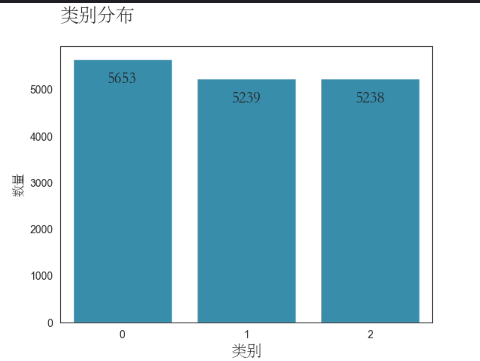
通过对以上打印的数据以及可视化的图片进行观察,我们可以看到三个类别的数量存在一定的差异。虽然数量上的差距不是太大,但对于训练学习结果可能会有一定的影响。为了克服类别不平衡的问题,我们可以采取一些方法来平衡数据集欠采样减少数量较多的类别的样本数量。
# 数据集欠采样
labels = np.array(labels)
paths = np.array(paths)
counter = Counter(labels)
print("原始样本数量:", counter)
cat_indices = np.where(labels == 0)[0]
dog_indices = np.where(labels == 1)[0]
wild_indices = np.where(labels == 2)[0]
min_samples = min([len(cat_indices), len(dog_indices), len(wild_indices)])
undersampled_cat_indices = resample(cat_indices, replace=False, n_samples=min_samples, random_state=42)
undersampled_dog_indices = resample(dog_indices, replace=False, n_samples=min_samples, random_state=42)
undersampled_wild_indices = resample(wild_indices, replace=False, n_samples=min_samples, random_state=42)
undersampled_indices = np.concatenate((undersampled_cat_indices, undersampled_dog_indices, undersampled_wild_indices))
undersampled_paths = paths[undersampled_indices]
undersampled_labels = labels[undersampled_indices]
counter_undersampled = Counter(undersampled_labels)
print("欠采样后的样本数量:", counter_undersampled)
counter_undersampled = Counter(undersampled_labels)
categories = [label_map[label] for label in counter_undersampled.keys()]
sample_counts = list(counter_undersampled.values())
# 可视化
sns.set_style("white")
plt.figure(figsize=(6.4, 4.8))
plot = sns.countplot(x=undersampled_labels, color='#2596be')
sns.despine()
plot.set_title('类别分布\n', x=0.1, y=1, font=font_prop,fontsize=18)
plot.set_ylabel("数量", x=0.02, font=font_prop, fontsize=12)
plot.set_xlabel("类别", font=font_prop, fontsize=15)

for p in plot.patches:
    plot.annotate(format(p.get_height(), '.0f'), (p.get_x() + p.get_width() / 2, p.get_height()),
                  ha='center', va='center', xytext=(0, -20), font=font_prop, textcoords='offset points', size=15)

plt.show()
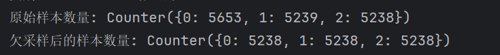

在进行欠采样后,每个类别的图片数量已经被扩展为一致的数量,使得模型在训练过程中更加公平地对待每个类别。
3、对数据进行预处理完之后,需要查看是否有缺失值,要检查路径和标签的数量是否匹配,并打印路径和标签数量,对缺失情况进行可视化
if len(undersampled_paths) != len(undersampled_labels):
    raise InvalidDatasetException(len(undersampled_paths), len(undersampled_labels))
#使用字符串格式化(f-string)来将整型值插入到字符串中。
print(f"打印paths列表的文件路径数量: {len(undersampled_paths)}")
print(f"打印labels列表的图片数量: {len(undersampled_labels)}")

# 缺失情况数据可视化
df = pd.DataFrame({'Path': undersampled_paths, 'Label': undersampled_labels})
missing_values = df.isnull().sum()
# 绘制条形图
plt.bar(missing_values.index, missing_values.values)
plt.xlabel("特征", fontproperties=font_prop, fontsize=12)
plt.ylabel("缺失值数量", fontproperties=font_prop, fontsize=12)
plt.title("缺失情况数据可视化", fontproperties=font_prop, fontsize=18)
plt.grid(False)
plt.xticks(rotation=90)
plt.show()
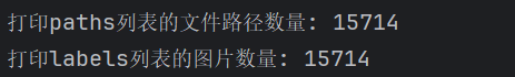
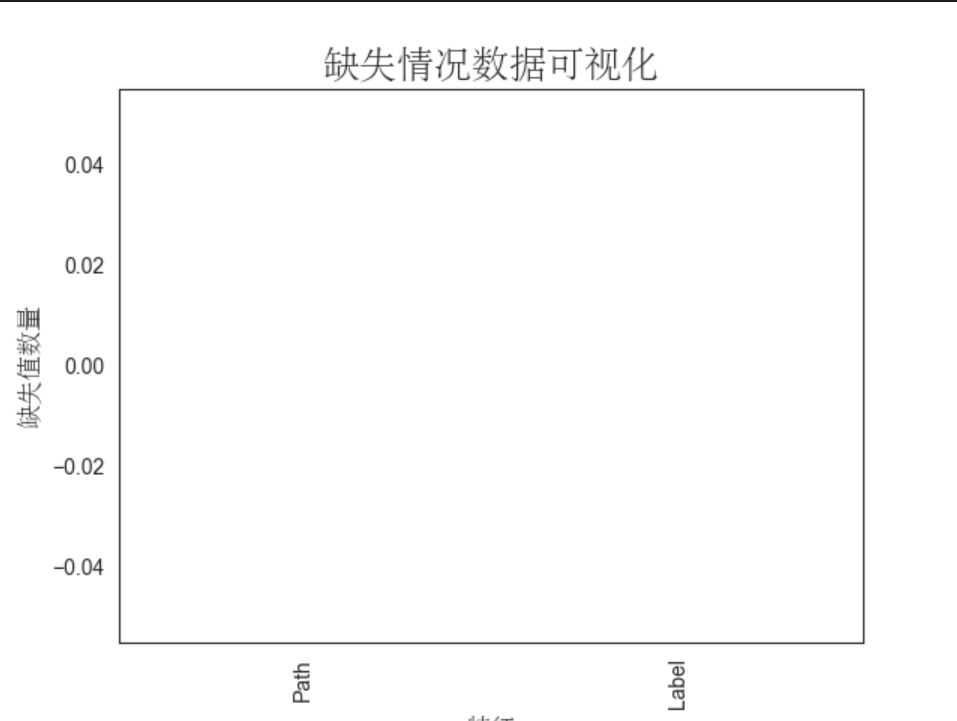
通过对打印的数据以及对条形图的查看,我们可以确认数据没有缺失。这意味着我们的数据集完整,并且可以进行进一步的分析和处理。
4、对将数据集划分为训练集和测试集,并创建对应的数据加载器,并定义了每个批次的样本数量。
dataset = AnimalDataset(undersampled_paths,undersampled_labels,(250,250))
from sklearn.model_selection import train_test_split
dataset_indices = list(range(0,len(dataset)))
#从数据集中划分训练集和测试集
train_indices,test_indices=train_test_split(dataset_indices,test_size=0.2,random_state=42)
print("训练集样本数量: ",len(train_indices))
print("测试集样本数量: ",len(test_indices))
#创建训练集和测试集的采样器
train_sampler = SubsetRandomSampler(train_indices)
test_sampler = SubsetRandomSampler(test_indices)
BATCH_SIZE = 128
train_loader = torch.utils.data.DataLoader(dataset, batch_size=BATCH_SIZE,
                                           sampler=train_sampler)
validation_loader = torch.utils.data.DataLoader(dataset, batch_size=BATCH_SIZE,
                                                sampler=test_sampler)
dataset[1][0].shape
images,labels = next(iter(train_loader))
type(labels)

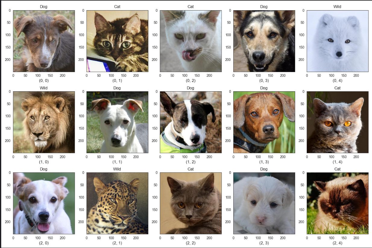
5、获取一个批次的训练数据,并可视化
def add_subplot_label(ax, label):
    ax.text(0.5, -0.15, label, transform=ax.transAxes,
            ha='center', va='center', fontsize=12)
images, labels = next(iter(train_loader))
fig, axis = plt.subplots(3, 5, figsize=(15, 10))
for i, ax in enumerate(axis.flat):
    with torch.no_grad():
        npimg = images[i].numpy()
        npimg = np.transpose(npimg, (1, 2, 0))
        label = label_map[int(labels[i])]
        ax.imshow(npimg)
        ax.set(title = f"{label}")
        ax.grid(False)
        add_subplot_label(ax, f"({i // axis.shape[1]}, {i % axis.shape[1]})")  # 添加编号
plt.tight_layout()
plt.show()
6、定义卷积神经网络模型,并设定在哪个设备上运行,为后续的模型训练做准备
class CNN(nn.Module):
    #定义了卷积神经网络的各个层和全连接层。
    def __init__(self):
        super(CNN, self).__init__()
        # First we'll define our layers
        self.conv1 = nn.Conv2d(3, 32, kernel_size=3, stride=2, padding=1)
        self.conv2 = nn.Conv2d(32, 64, kernel_size=3, stride=2, padding=1)
        self.batchnorm1 = nn.BatchNorm2d(64)
        self.conv3 = nn.Conv2d(64, 128, kernel_size=3, stride=2, padding=1)
        self.batchnorm2 = nn.BatchNorm2d(128)
        self.conv4 = nn.Conv2d(128, 256, kernel_size=3, stride=2, padding=1)
        self.batchnorm3 = nn.BatchNorm2d(256)
        self.maxpool = nn.MaxPool2d(2, 2)
        self.fc1 = nn.Linear(256 * 2 * 2, 512)
        self.fc2 = nn.Linear(512, 3)
    #定义数据在模型中的流动
    def forward(self, x):
        x = F.relu(self.conv1(x))
        x = F.relu(self.conv2(x))
        x = self.batchnorm1(x)
        x = self.maxpool(x)
        x = F.relu(self.conv3(x))
        x = self.batchnorm2(x)
        x = self.maxpool(x)
        x = F.relu(self.conv4(x))
        x = self.batchnorm3(x)
        x = self.maxpool(x)
        x = x.view(-1, 256 * 2 * 2)
        x = self.fc1(x)
        x = self.fc2(x)
        x = F.log_softmax(x, dim=1)
        return x
#选择模型运行的设备
device = torch.device("cuda" if torch.cuda.is_available() else "cpu")
device
7、执行模型的训练过程,使用交叉熵损失函数和RMSprop优化器来定义损失计算和参数优化的方法,设置了训练的轮次数,并记录每个训练轮次的损失和准确率,对每个训练轮次的损失和准确率进行可视化
model = CNN().to(device)
criterion = nn.CrossEntropyLoss()
optimizer = optim.RMSprop(model.parameters(),lr=1e-4)
EPOCH_NUMBER =6
TRAIN_LOSS = []
TRAIN_ACCURACY = []
#训练过程
for epoch in range(1, EPOCH_NUMBER + 1):
    epoch_loss = 0.0
    correct = 0
    total = 0
    #遍历训练数据加载器
    for data_, target_ in train_loader:
        target_ = target_.to(device)
        data_ = data_.to(device)
        #清零优化器中之前的梯度,准备计算当前轮次的梯度。
        optimizer.zero_grad()
        #将输入数据传递给模型,获取模型的预测输出。
        outputs = model(data_)
        loss = criterion(outputs, target_)
        loss.backward()
        optimizer.step()
        epoch_loss = epoch_loss + loss.item()
        _, pred = torch.max(outputs, dim=1)
        #统计预测正确的样本数量,将预测值与真实标签进行比较,并累计正确预测的数量。
        correct = correct + torch.sum(pred == target_).item()
        total += target_.size(0)
        #记录每个训练轮次的损失和准确率,并输出当前训练轮次的准确率和损失。
    TRAIN_LOSS.append(epoch_loss)
    TRAIN_ACCURACY.append(100 * correct / total)
    print(f"Epoch {epoch}: Accuracy: {100 * correct / total}, Loss: {epoch_loss}")
#可视化训练过程中的损失和准确率
plt.subplots(figsize=(6, 4))
plt.plot(range(EPOCH_NUMBER), TRAIN_LOSS, color="blue", label="Loss")
plt.legend()
plt.xlabel("轮次", fontproperties=font_prop)
plt.ylabel("损失值", fontproperties=font_prop)
plt.title("训练损失", fontproperties=font_prop)
plt.show()
plt.subplots(figsize=(6, 4))
plt.plot(range(EPOCH_NUMBER), TRAIN_ACCURACY, color="green", label="Accuracy")
plt.legend()
plt.xlabel("轮次", fontproperties=font_prop)
plt.ylabel("准确率", fontproperties=font_prop)
plt.title("训练准确率", fontproperties=font_prop)
plt.show()
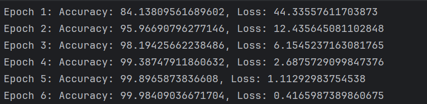
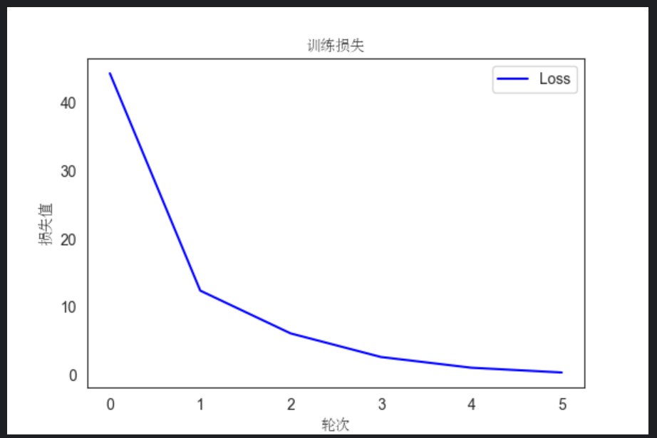
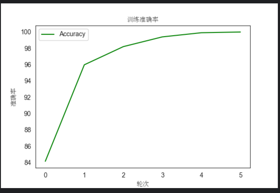
通过上面的数据以及图形,我们可以观察到,随着训练轮次的增加,训练损失逐渐降低,训练准确率逐渐提高。这表明模型在学习过程中逐渐减小了预测值与真实标签之间的差异,提高了对训练数据的拟合能力。每轮的训练损失率都比上一轮的损失率低,说明模型的优化算法有效地调整了参数,使模型逐渐逼近最优解。也意味着模型在训练数据上的分类性能不断改善,更准确地预测了样本的标签。每轮的训练准确率都比上一轮的高,说明模型逐渐学习到了更多的特征和模式,提高了对训练数据的分类准确性。总体来说损失下降和准确率提高是我们期望在训练过程中看到的趋势,表明模型正在逐渐优化和提升性能。
8、评估模型在每个类别上的性能,并绘制ROC曲线以衡量模型的分类准确性
def predict_labels(model, data_loader):
    model.eval()
    y_pred = []
    y_true = []
    with torch.no_grad():
        for images, labels in data_loader:
            outputs = model(images)
            _, predicted = torch.max(outputs.data, 1)
            y_pred.extend(predicted.numpy())
            y_true.extend(labels.numpy())
    return y_pred, y_true
# 获取预测结果
y_pred, y_true = predict_labels(model, validation_loader)
# 计算每个类别的ROC曲线
fpr = dict()
tpr = dict()
roc_auc = dict()
num_classes = len(label_map)
for i in range(num_classes):
    fpr[i], tpr[i], _ = roc_curve((np.array(y_true) == i).astype(int), (np.array(y_pred) == i).astype(int))
    roc_auc[i] = auc(fpr[i], tpr[i])
# 绘制ROC曲线
plt.figure(figsize=(10, 8))
colors = ['b', 'g', 'r']  # 每个类别的曲线颜色
for i in range(num_classes):
    plt.plot(fpr[i], tpr[i], color=colors[i], lw=2, label='类别 {0} 的ROC曲线 (AUC = {1:.2f})'.format(i, roc_auc[i]))
plt.plot([0, 1], [0, 1], color='navy', lw=2, linestyle='--')
plt.xlim([0.0, 1.0])
plt.ylim([0.0, 1.05])
plt.xlabel('假阳性率', fontproperties=font_prop)
plt.ylabel('真阳性率', fontproperties=font_prop)
plt.title('接收者操作特征曲线', fontproperties=font_prop)
plt.legend(loc="lower right", prop=font_prop)
plt.show()
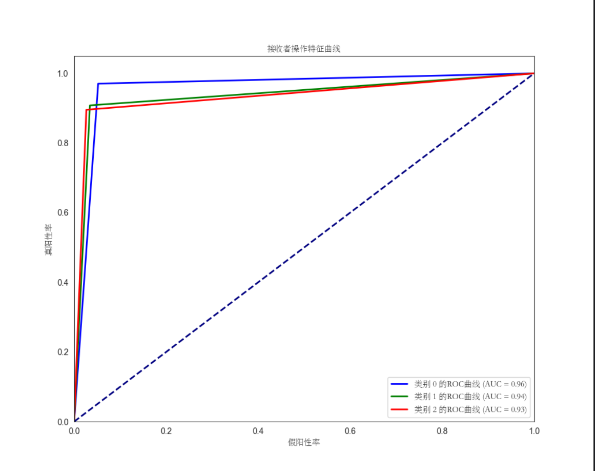
从图片中可以看出来,cat类别的ROC曲线相对于其他类别的曲线更加接近左上角,而dog和wild类别的曲线则相对较低。这意味着在不同的阈值下,模型更容易将cat类别正确分类为正例,并且在cat类别上具有较高的真阳性率和较低的假阳性率。相比之下,dog和wild类别在模型分类能力方面相对较弱,表明模型更容易将它们错误地分类为其他类别。
9、评估模型在验证集上对模型进行测试,并计算评估指标(准确率、精确率、召回率)以及混淆矩阵,并使用可视化工具将混淆矩阵进行可视化。
model.eval() # 将模型设置为评估模式
predictions = [] # 存储预测结果和真实标签
true_labels = []
# 使用测试集进行预测
with torch.no_grad():
    for images, labels in validation_loader:
        images = images.to(device)
        labels = labels.to(device)
        outputs = model(images) # 前向传播
        _, predicted = torch.max(outputs.data, 1)  # 获取预测结果
        predictions.extend(predicted.tolist())    # 存储预测结果和真实标签
        true_labels.extend(labels.tolist())
# 将预测结果和真实标签转换为NumPy数组
predictions = np.array(predictions)
true_labels = np.array(true_labels)
accuracy = accuracy_score(true_labels, predictions) # 计算准确率
precision = precision_score(true_labels, predictions, average='macro') # 计算精确率
recall = recall_score(true_labels, predictions, average='macro') # 计算召回率
confusion = confusion_matrix(true_labels, predictions) # 计算混淆矩阵
# 打印评估结果
print("准确率:", accuracy)
print("精确率:", precision)
print("召回率:", recall)
print("混淆矩阵:")
print(confusion)
# 可视化混淆矩阵
labels = ['Cat', 'Dog', 'Wild']
plt.rcParams['font.sans-serif'] = ['STFangsong']
plt.figure(figsize=(8, 6))
sns.heatmap(confusion, annot=True, fmt="d", cmap="Blues", xticklabels=labels, yticklabels=labels)
plt.xlabel('预测标签')
plt.ylabel('真实标签')
plt.title('混淆矩阵')
plt.show()
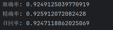
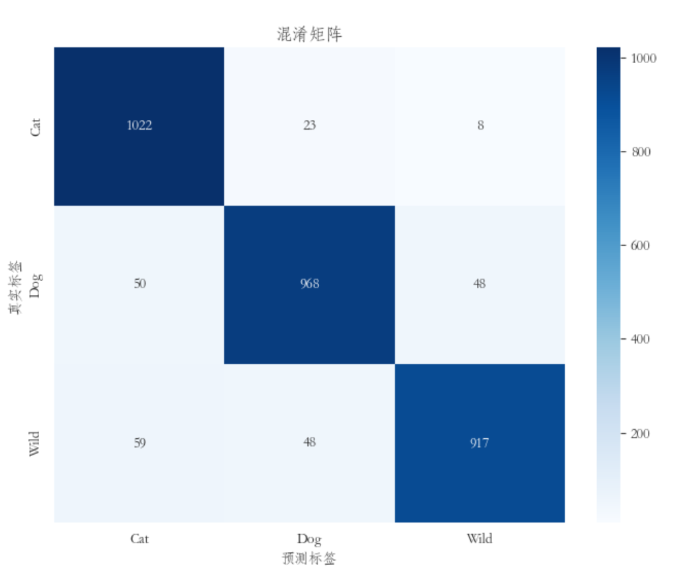
通过准确率、精准率、召回率可以得出模型在整体预测能力上表现良好,准确率较高。同时,模型在区分正例和负例方面也有较好的表现,具有较高的精确率和召回率。通过对混淆矩阵图的查看可以得出,在cat类别上,主对角线上的数值相对较高,而在dog和wild类别上较低,那么可以推断模型在cat类别上的识别率较高,而在dog和wild类别上的识别率较低。
 四、总结
  对于本次的机器学习,我觉得完成得还是较为不错,模型在整体预测能力上表现良好,随着训练轮次的增加,训练损失逐渐降低,训练准确率逐渐提高,也符合了我对于模型的预期,表明模型正在逐步优化和改善性能。
  也了解到当训练数据中的不同类别之间存在明显的数量差异时,模型倾向于偏向数量较多的类别,导致对数量较少的类别预测能力下降,需要通过合适的处理方法和技术,有效地解决这个问题,提高模型的性能和泛化能力。
  模型在对于dog类和wild类的识别率较低的问题,还需要进一步的通过增加模型的层数、调整卷积核的大小、增加正则化等方法对模型进行改善。

完整代码如下:
import pandas as pd
from PIL import Image
import torch.nn as nn
import torch.optim as optim
from torch.utils.data.sampler import SubsetRandomSampler
from torch.utils.data import Dataset
import torchvision.transforms as transforms
import matplotlib.font_manager as fm
import torch
import torch.nn.functional as F
from sklearn.metrics import accuracy_score, precision_score, recall_score, confusion_matrix
import matplotlib.pyplot as plt
import seaborn as sns
from collections import Counter
from sklearn.utils import resample
import numpy as np
#设置全局字体为华文仿宋
plt.rcParams['font.sans-serif'] = ['STFangsong']
# 定义一个自定义异常类,用于在数据集路径数量和标签数量不兼容时引发异常
class InvalidDatasetException(Exception):
    def __init__(self, len_of_paths, len_of_labels):
        super().__init__(
            f"Number of paths ({len_of_paths}) is not compatible with number of labels ({len_of_labels})"
        )
transform = transforms.Compose([transforms.ToTensor()])
#定义一个数据集类,包含了图像路径、图像标签和图像大小的信息,并在构造函数中检查图像路径和图像标签的数量是否匹配,如果不匹配则引发异常。
class AnimalDataset(Dataset):
    def __init__(self, img_paths, img_labels, size_of_images):
        self.img_paths = img_paths
        self.img_labels = img_labels
        self.size_of_images = size_of_images
        if len(self.img_paths) != len(self.img_labels):
            raise InvalidDatasetException(self.img_paths, self.img_labels)
    # 获取数据集的大小
    def __len__(self):
        return len(self.img_paths)
    #获取数据集中的一个样本,将图像数据转换为张量,并同时返回对应的标签
    def __getitem__(self, index):
        PIL_IMAGE = Image.open(self.img_paths[index]).resize(self.size_of_images)
        TENSOR_IMAGE = transform(PIL_IMAGE)
        label = self.img_labels[index]
        return TENSOR_IMAGE, label
import glob
#数据预处理
paths = []
labels = []
label_map = {0: "Cat",
             1: "Dog",
             2: "Wild"
             }
# 处理Cat类别
cat_paths = glob.glob("D:/edge下载/archive/afhq/train/cat/*") + glob.glob("D:/edge下载/archive/afhq/val/cat/*")
for cat_path in cat_paths:
    paths.append(cat_path)
    labels.append(0)
# 处理Dog类别
dog_paths = glob.glob("D:/edge下载/archive/afhq/train/dog/*") + glob.glob("D:/edge下载/archive/afhq/val/dog/*")
for dog_path in dog_paths:
    paths.append(dog_path)
    labels.append(1)
# 处理Wild类别
wild_paths = glob.glob("D:/edge下载/archive/afhq/train/wild/*") + glob.glob("D:/edge下载/archive/afhq/val/wild/*")
for wild_path in wild_paths:
    paths.append(wild_path)
    labels.append(2)
# 创建包含类别信息的数据框
data = pd.DataFrame({'classes': labels})
# 打印总类别数和每个类别的数量
num_classes = len(label_map)
print('总类别数:', num_classes)
for class_label, class_name in label_map.items():
    count = data[data['classes'] == class_label].shape[0]
    print(f"类别 {class_name}: {count} 张照片")
font_path = "C:/Windows/Fonts/STSONG.TTF"
font_prop = fm.FontProperties(fname=font_path)
# 绘制类别分布的计数图
sns.set_style("white")
plot = sns.countplot(x=data['classes'], color='#2596be')
plt.figure(figsize=(15, 12))
sns.despine()
plot.set_title('类别分布\n', x=0.1, y=1, font=font_prop, fontsize=18)
plot.set_ylabel("数量", x=0.02, font=font_prop, fontsize=12)
plot.set_xlabel("类别", font=font_prop, fontsize=15)
for p in plot.patches:
    plot.annotate(format(p.get_height(), '.0f'), (p.get_x() + p.get_width() / 2, p.get_height()),
                  ha='center', va='center', xytext=(0, -20), font=font_prop, textcoords='offset points', size=15)
plt.show()

# 数据集欠采样
labels = np.array(labels)
paths = np.array(paths)
counter = Counter(labels)
print("原始样本数量:", counter)
cat_indices = np.where(labels == 0)[0]
dog_indices = np.where(labels == 1)[0]
wild_indices = np.where(labels == 2)[0]
min_samples = min([len(cat_indices), len(dog_indices), len(wild_indices)])
undersampled_cat_indices = resample(cat_indices, replace=False, n_samples=min_samples, random_state=42)
undersampled_dog_indices = resample(dog_indices, replace=False, n_samples=min_samples, random_state=42)
undersampled_wild_indices = resample(wild_indices, replace=False, n_samples=min_samples, random_state=42)
undersampled_indices = np.concatenate((undersampled_cat_indices, undersampled_dog_indices, undersampled_wild_indices))
undersampled_paths = paths[undersampled_indices]
undersampled_labels = labels[undersampled_indices]
counter_undersampled = Counter(undersampled_labels)
print("欠采样后的样本数量:", counter_undersampled)
counter_undersampled = Counter(undersampled_labels)
categories = [label_map[label] for label in counter_undersampled.keys()]
sample_counts = list(counter_undersampled.values())
# 可视化
sns.set_style("white")
plt.figure(figsize=(6.4, 4.8))
plot = sns.countplot(x=undersampled_labels, color='#2596be')
sns.despine()
plot.set_title('类别分布\n', x=0.1, y=1, font=font_prop,fontsize=18)
plot.set_ylabel("数量", x=0.02, font=font_prop, fontsize=12)
plot.set_xlabel("类别", font=font_prop, fontsize=15)

for p in plot.patches:
    plot.annotate(format(p.get_height(), '.0f'), (p.get_x() + p.get_width() / 2, p.get_height()),
                  ha='center', va='center', xytext=(0, -20), font=font_prop, textcoords='offset points', size=15)

plt.show()

# 检查数据缺失
if len(undersampled_paths) != len(undersampled_labels):
    raise InvalidDatasetException(len(undersampled_paths), len(undersampled_labels))
#使用字符串格式化(f-string)来将整型值插入到字符串中。
print(f"打印paths列表的文件路径数量: {len(undersampled_paths)}")
print(f"打印labels列表的图片数量: {len(undersampled_labels)}")

# 缺失情况数据可视化
df = pd.DataFrame({'Path': undersampled_paths, 'Label': undersampled_labels})
missing_values = df.isnull().sum()
# 绘制条形图
plt.bar(missing_values.index, missing_values.values)
plt.xlabel("特征", fontproperties=font_prop, fontsize=12)
plt.ylabel("缺失值数量", fontproperties=font_prop, fontsize=12)
plt.title("缺失情况数据可视化", fontproperties=font_prop, fontsize=18)
plt.grid(False)
plt.xticks(rotation=90)
plt.show()

dataset = AnimalDataset(undersampled_paths,undersampled_labels,(250,250))
from sklearn.model_selection import train_test_split
dataset_indices = list(range(0,len(dataset)))
#从数据集中划分训练集和测试集
train_indices,test_indices=train_test_split(dataset_indices,test_size=0.2,random_state=42)
print("训练集样本数量: ",len(train_indices))
print("测试集样本数量: ",len(test_indices))
#创建训练集和测试集的采样器
train_sampler = SubsetRandomSampler(train_indices)
test_sampler = SubsetRandomSampler(test_indices)
BATCH_SIZE = 128
train_loader = torch.utils.data.DataLoader(dataset, batch_size=BATCH_SIZE,
                                           sampler=train_sampler)
validation_loader = torch.utils.data.DataLoader(dataset, batch_size=BATCH_SIZE,
                                                sampler=test_sampler)
dataset[1][0].shape
images,labels = next(iter(train_loader))
type(labels)
def add_subplot_label(ax, label):
    ax.text(0.5, -0.15, label, transform=ax.transAxes,
            ha='center', va='center', fontsize=12)
#来获取一个批次的训练数据,并将其可视化
images, labels = next(iter(train_loader))
fig, axis = plt.subplots(3, 5, figsize=(15, 10))
for i, ax in enumerate(axis.flat):
    with torch.no_grad():
        npimg = images[i].numpy()
        npimg = np.transpose(npimg, (1, 2, 0))
        label = label_map[int(labels[i])]
        ax.imshow(npimg)
        ax.set(title = f"{label}")
        ax.grid(False)
        add_subplot_label(ax, f"({i // axis.shape[1]}, {i % axis.shape[1]})")  # 添加编号
plt.tight_layout()
plt.show()
#定义卷积神经网络模型
class CNN(nn.Module):
    #定义了卷积神经网络的各个层和全连接层。
    def __init__(self):
        super(CNN, self).__init__()
        # First we'll define our layers
        self.conv1 = nn.Conv2d(3, 32, kernel_size=3, stride=2, padding=1)
        self.conv2 = nn.Conv2d(32, 64, kernel_size=3, stride=2, padding=1)
        self.batchnorm1 = nn.BatchNorm2d(64)
        self.conv3 = nn.Conv2d(64, 128, kernel_size=3, stride=2, padding=1)
        self.batchnorm2 = nn.BatchNorm2d(128)
        self.conv4 = nn.Conv2d(128, 256, kernel_size=3, stride=2, padding=1)
        self.batchnorm3 = nn.BatchNorm2d(256)
        self.maxpool = nn.MaxPool2d(2, 2)
        self.fc1 = nn.Linear(256 * 2 * 2, 512)
        self.fc2 = nn.Linear(512, 3)
    #定义数据在模型中的流动
    def forward(self, x):
        x = F.relu(self.conv1(x))
        x = F.relu(self.conv2(x))
        x = self.batchnorm1(x)
        x = self.maxpool(x)
        x = F.relu(self.conv3(x))
        x = self.batchnorm2(x)
        x = self.maxpool(x)
        x = F.relu(self.conv4(x))
        x = self.batchnorm3(x)
        x = self.maxpool(x)
        x = x.view(-1, 256 * 2 * 2)
        x = self.fc1(x)
        x = self.fc2(x)
        x = F.log_softmax(x, dim=1)
        return x
#选择模型运行的设备
device = torch.device("cuda" if torch.cuda.is_available() else "cpu")
device
#设置和初始化将用于模型训练过程,记录每个训练轮次的损失和准确率
model = CNN().to(device)
criterion = nn.CrossEntropyLoss()
optimizer = optim.RMSprop(model.parameters(),lr=1e-4)
EPOCH_NUMBER =6
TRAIN_LOSS = []
TRAIN_ACCURACY = []
#训练过程
for epoch in range(1, EPOCH_NUMBER + 1):
    epoch_loss = 0.0
    correct = 0
    total = 0
    #遍历训练数据加载器
    for data_, target_ in train_loader:
        target_ = target_.to(device)
        data_ = data_.to(device)
        #清零优化器中之前的梯度,准备计算当前轮次的梯度。
        optimizer.zero_grad()
        #将输入数据传递给模型,获取模型的预测输出。
        outputs = model(data_)
        target_ = target_.long()
        loss = criterion(outputs, target_)
        loss.backward()
        optimizer.step()
        epoch_loss = epoch_loss + loss.item()
        _, pred = torch.max(outputs, dim=1)
        #统计预测正确的样本数量,将预测值与真实标签进行比较,并累计正确预测的数量。
        correct = correct + torch.sum(pred == target_).item()
        total += target_.size(0)
        #记录每个训练轮次的损失和准确率,并输出当前训练轮次的准确率和损失。
    TRAIN_LOSS.append(epoch_loss)
    TRAIN_ACCURACY.append(100 * correct / total)
    print(f"Epoch {epoch}: Accuracy: {100 * correct / total}, Loss: {epoch_loss}")
#可视化训练过程中的损失和准确率
plt.subplots(figsize=(6, 4))
plt.plot(range(EPOCH_NUMBER), TRAIN_LOSS, color="blue", label="Loss")
plt.legend()
plt.xlabel("轮次", fontproperties=font_prop)
plt.ylabel("损失值", fontproperties=font_prop)
plt.title("训练损失", fontproperties=font_prop)
plt.show()
plt.subplots(figsize=(6, 4))
plt.plot(range(EPOCH_NUMBER), TRAIN_ACCURACY, color="green", label="Accuracy")
plt.legend()
plt.xlabel("轮次", fontproperties=font_prop)
plt.ylabel("准确率", fontproperties=font_prop)
plt.title("训练准确率", fontproperties=font_prop)
plt.show()

from sklearn.metrics import roc_curve, auc
# 预测测试集的标签
def predict_labels(model, data_loader):
    model.eval()
    y_pred = []
    y_true = []
    with torch.no_grad():
        for images, labels in data_loader:
            outputs = model(images)
            _, predicted = torch.max(outputs.data, 1)
            y_pred.extend(predicted.numpy())
            y_true.extend(labels.numpy())
    return y_pred, y_true
# 获取预测结果
y_pred, y_true = predict_labels(model, validation_loader)
# 计算每个类别的ROC曲线
fpr = dict()
tpr = dict()
roc_auc = dict()
num_classes = len(label_map)
for i in range(num_classes):
    fpr[i], tpr[i], _ = roc_curve((np.array(y_true) == i).astype(int), (np.array(y_pred) == i).astype(int))
    roc_auc[i] = auc(fpr[i], tpr[i])
# 绘制ROC曲线
plt.figure(figsize=(10, 8))
colors = ['b', 'g', 'r']  # 每个类别的曲线颜色
for i in range(num_classes):
    plt.plot(fpr[i], tpr[i], color=colors[i], lw=2, label='类别 {0} 的ROC曲线 (AUC = {1:.2f})'.format(i, roc_auc[i]))
plt.plot([0, 1], [0, 1], color='navy', lw=2, linestyle='--')
plt.xlim([0.0, 1.0])
plt.ylim([0.0, 1.05])
plt.xlabel('假阳性率', fontproperties=font_prop)
plt.ylabel('真阳性率', fontproperties=font_prop)
plt.title('接收者操作特征曲线', fontproperties=font_prop)
plt.legend(loc="lower right", prop=font_prop)
plt.show()

model.eval() # 将模型设置为评估模式
predictions = [] # 存储预测结果和真实标签
true_labels = []
# 使用测试集进行预测
with torch.no_grad():
    for images, labels in validation_loader:
        images = images.to(device)
        labels = labels.to(device)
        outputs = model(images) # 前向传播
        _, predicted = torch.max(outputs.data, 1)  # 获取预测结果
        predictions.extend(predicted.tolist())    # 存储预测结果和真实标签
        true_labels.extend(labels.tolist())
# 将预测结果和真实标签转换为NumPy数组
predictions = np.array(predictions)
true_labels = np.array(true_labels)
accuracy = accuracy_score(true_labels, predictions) # 计算准确率
precision = precision_score(true_labels, predictions, average='macro') # 计算精确率
recall = recall_score(true_labels, predictions, average='macro') # 计算召回率
confusion = confusion_matrix(true_labels, predictions) # 计算混淆矩阵
# 打印评估结果
print("准确率:", accuracy)
print("精确率:", precision)
print("召回率:", recall)
print("混淆矩阵:")
print(confusion)
# 可视化混淆矩阵
labels = ['Cat', 'Dog', 'Wild']
plt.rcParams['font.sans-serif'] = ['STFangsong']
plt.figure(figsize=(8, 6))
sns.heatmap(confusion, annot=True, fmt="d", cmap="Blues", xticklabels=labels, yticklabels=labels)
plt.xlabel('预测标签')
plt.ylabel('真实标签')
plt.title('混淆矩阵')
plt.show()