summer pocket_久岛鸥我将会跨越七大洋，将我的爱意带到你的身边

线性回归基本概念

这里的price泛化后就是我们的y，即标签label
这里的area,age泛化后就是我们的X，即特征features

当L（W，b）能够通过直接求导得到W与b,那么我们称之W与b有解析解（因为L（W,b）是一个凸函数，当求导后令导数为0,求出的W与b就是使得L（w,b）最小的参数）

这里公式上的n为学习率，他是代表在梯度方向上走的“步长”
后面看起来比较复杂的导数其实是在说明

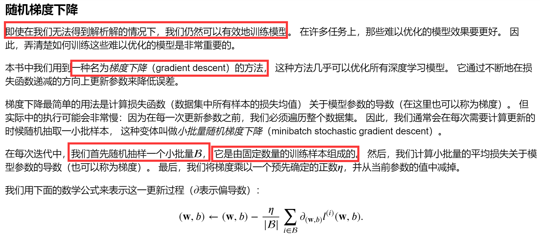
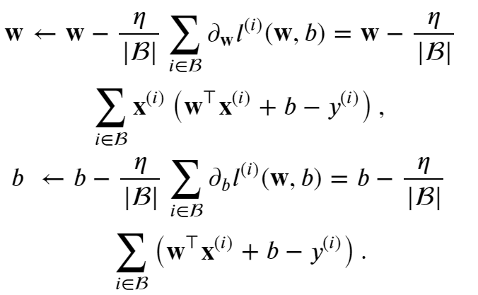
梯度是指函数数值增长最大的方向
当梯度前面有负号，则是说明指向函数数值减少最大的方向
上面的操作都是让参数w与b向着让L（W，b）最大减少的方向变化的

线性回归的从零开始实现

生成数据集
读取数据集
初始化模型参数
定义模型
定义损失函数
定义优化算法
训练

上述过程是一般的深度学习的一般过程
因为我们没有数据，需要用正则表达式函数创建数据所以有生成数据集这个步骤

生成数据集

%matplotlib inline
import random
import torch
from d2l import torch as d2l

#生成数据，这里模拟出来的是真实的y,x
def synthetic_data(w, b, num_examples):  #@save
    """生成y=Xw+b+噪声"""
    X = torch.normal(0, 1, (num_examples, len(w))) 
    y = torch.matmul(X, w) + b
    y += torch.normal(0, 0.01, y.shape)
    return X, y.reshape((-1, 1))

true_w = torch.tensor([2, -3.4])
true_b = 4.2
#一共模拟出1000个点，得到X=features(特征)，Y=labels(标签)
features, labels = synthetic_data(true_w, true_b, 1000)

# 画出上述生成的数据
d2l.set_figsize()
d2l.plt.scatter(features[:, 0].detach().numpy(), labels.detach().numpy(), 1);
d2l.plt.scatter(features[:, 1].detach().numpy(), labels.detach().numpy(), 1);

这一步中我们先设定出W与b，然后利用随机函数求出X，利用y=WX+b求出y
下面我们可以利用得出的数据X，y进行线性回归，用线性回归得出的W与b,和我们设置的W与b进行比较，差距越小，说明线性回归的效果越好

读取数据集

'''
训练模型时要对数据集进行遍历，每次抽取一小批量样本，并使用它们来更新我们的模型。 
由于这个过程是训练机器学习算法的基础，所以有必要定义一个函数， 该函数能打乱数据集中的样本并以小批量方式获取数据。
'''
# 读取数据
# 这个函数的作用就真是每一次从features和labels中随机取出batch_size个数据点出来
def data_iter(batch_size,features,labels):
    num_examples=len(features)
    print(f'len(features):{len(features)}\n')
    indices=list(range(num_examples))
    random.shuffle(indices)
    for i in range(0,num_examples,batch_size):
        batch_indices=torch.tensor(
            indices[i:min(i+batch_size,num_examples)])
        yield features[batch_indices],labels[batch_indices]

batch_size = 10

range函数：range(start, stop[, step])

令人震惊的是 features[batch_indices] , labels[batch_indices] 的用法，居然可以使用张量batch_indices作为下标一次取多个值

num_examples=len(features): features是个矩阵，len(features)得出的是其行数

batch_indices=torch.tensor(indices[i:min(i+batch_size,num_examples)]) 其中i:min(i+batch_size,num_examples)利用的是切片技术

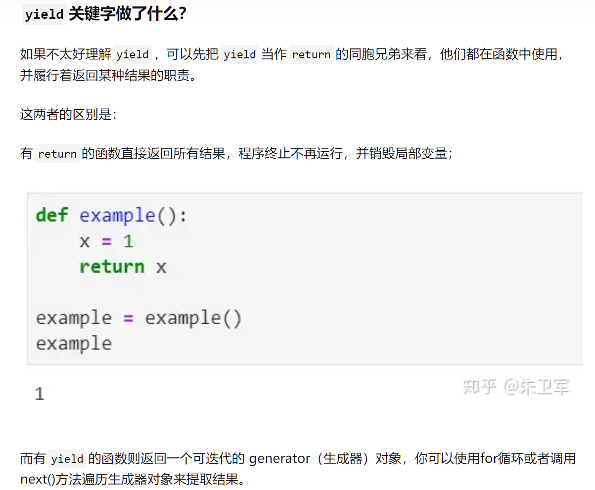
yield：
就是可以简单地理解为yield是用来返回的，但是返回后函数中的状态不会销毁，下次使用next()或for再次执行时，可以接着原来的状态继续执行

如：

for X, y in data_iter(batch_size, features, labels):
    print(X, '\n', y)
    break

上述就是调用函数的一种方式

初始化模型参数

# 初始化模型参数
w=torch.normal(0,0.01,size=(2,1),requires_grad=True)
b=torch.zeros(1,requires_grad=True)

定义模型

#定义模型
def linreg(X,w,b): #@save
    return torch.matmul(X,w)+b

定义损失函数

# 定义损失函数
def squared_loss(y_hat,y):#@save
    return (y_hat-y.reshape(y_hat.shape))**2/2

定义优化算法

# 定义优化算法
#batch_size为样本个数
def sgd(params,lr,batch_size):#@save
    with torch.no_grad():
        for param in params:
            param -= lr*param.grad/batch_size
            param.grad.zero_()

训练

# 训练

# 先定义参数
lr=0.03 #学习率
num_epochs=3 #训练次数
net=linreg
loss=squared_loss

for epoch in range(num_epochs):
    for X,y in data_iter(batch_size,features,labels):
        l=loss(net(X,w,b),y)
        l.sum().backward()
        sgd([w,b],lr,batch_size)
    with torch.no_grad():
        train_l=loss(net(features,w,b),labels)
        print(f'epoch {epoch+1},loss {float(train_l.mean()):f}')