简单线性回归 - 用一元线性回归建立披萨的大小和价格的关系,然后进行预测
披萨数据:
| 编号 | 直径英寸 | 价格美元 |
|---|---|---|
| 1 | 6 | 7 |
| 2 | 8 | 9 |
| 3 | 10 | 13 |
| 4 | 14 | 17.5 |
| 5 | 18 | 18 |
观察数据
# 引入numpy matplotlib模块
import numpy as np
import matplotlib.pyplot as plt
# 输入披萨数据
X = np.array([[6],[8],[10],[14],[18]])
y = [ 7 , 9, 13, 17.5, 18]
X
array([[ 6],
       [ 8],
       [10],
       [14],
       [18]])
y
[7, 9, 13, 17.5, 18]
# 设置中文字体
plt.rcParams['font.sans-serif'] = ['SimHei']  # 指定默认字体
plt.rcParams['axes.unicode_minus'] = False  # 解决保存图像是负号'-'显示为方块的问题
# 设置画布大小
plt.rcParams['figure.figsize'] = (8, 6)
import matplotlib.pyplot as plt

plt.scatter(X,y,color = 'red')
plt.xlabel('披萨直径')
plt.ylabel('披萨价格')
plt.title('披萨定价:直径与价格关系图')
plt.show()
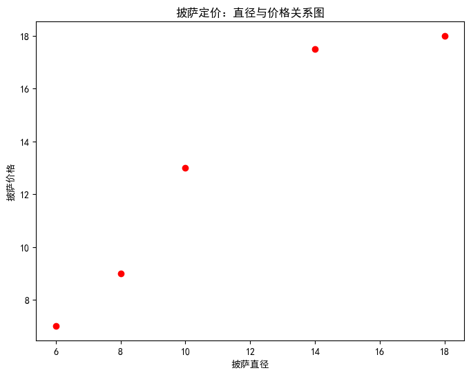
结论:
观察可知,直径增加,披萨用料增加,价格随之升高,
训练线性回归模型
# 引入scikit-learn
# sklearn, scikit-learn
from sklearn.linear_model import LinearRegression
# 创建一个空的线性回归估计器, 空的模型,参数是空的
model = LinearRegression()
# 训练模型
model.fit( X, y )
LinearRegression()In a Jupyter environment, please rerun this cell to show the HTML representation or trust the notebook.
On GitHub, the HTML representation is unable to render, please try loading this page with nbviewer.org.
LinearRegression()
y = b0 + b1*X
# 查看参数, coefficients, b1斜率
model.coef_
array([0.9762931])
# 查看截距 interception
model.intercept_
1.965517241379315
np.arange(1,25)
array([ 1,  2,  3,  4,  5,  6,  7,  8,  9, 10, 11, 12, 13, 14, 15, 16, 17,
       18, 19, 20, 21, 22, 23, 24])
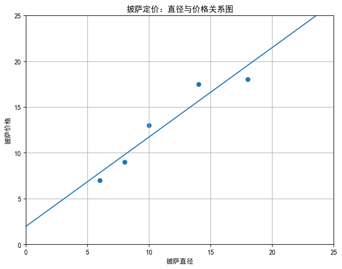
# 回归模型可视化
plt.figure()
plt.scatter(X,y)

plt.plot(np.arange(0,25), model.predict(np.arange(0,25).reshape(-1,1)),'-')
plt.grid(True)
plt.xlim([5,20])
plt.axis([0,25,0,25])
plt.xlabel('披萨直径')
plt.ylabel('披萨价格')
plt.title('披萨定价:直径与价格关系图')
plt.show()
# 拟合优度 R^2
model.score(X,y)
0.9100015964240102
预测
预测直径=12寸的披萨价格
# 预测直径 = 12 的披萨价格
model.predict([[12]]).round(0)
array([14.])
了解残差平方和RSS、损失函数 Loss Function
损失即代价,损失函数用来衡量一个模型的误差,所谓误差是真实值与预测值的距离。

误差也叫残差,error。模型的残差是真实观察值的点到回归直线或回归超平面之间的垂直线
# 回归模型可视化
y_pred = model.predict(X).reshape(-1,1)
# plt.figure()
plt.scatter(X,y)
plt.plot(np.arange(0,25), model.predict(np.arange(0,25).reshape(-1,1)),'-',color = 'black')

for i in range(len(X)):
    plt.plot([X[i],X[i]], [y[i],y_pred[i]])
    # plt.scatter([X[i],X[i]], [y[i],y_pred[i]])

plt.grid(True)
plt.xlim([5,20])
plt.axis([0,25,0,25])
plt.xlabel('披萨直径')
plt.ylabel('披萨价格')
plt.title('披萨定价:直径与价格关系图')
plt.show()
D:\ProgramData\Miniconda3\lib\site-packages\numpy\core\shape_base.py:65: VisibleDeprecationWarning: Creating an ndarray from ragged nested sequences (which is a list-or-tuple of lists-or-tuples-or ndarrays with different lengths or shapes) is deprecated. If you meant to do this, you must specify 'dtype=object' when creating the ndarray.
  ary = asanyarray(ary)
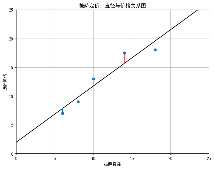
OLS最小二乘法的损失函数是残差平方和RSS

RSS通过以下代码可以计算得到:
# 计算残差平方和
np.sum((model.predict(X) - y)**2).round(2)
8.75
模型评估
一元线性回归采用 R^2 评估回归效果
RSS = np.sum((model.predict(X) - y)**2)
TSS = np.sum((y - np.mean(y))**2)
print(RSS)
print(TSS)
8.747844827586203
97.19999999999999


公式:
R^2 = 1 - RSS/TSS
R_squared = 1-RSS/TSS
print(R_squared)
0.9100015964240102
# 检查模型AUC值,与R^2是一样的
print(model.score(X,y))
0.9100015964240102
测试一组新数据用于验证模型
新样本数据如下:
| 序号 | 直径 | 价格 |
|---|---|---|
| 1 | 8 | 11 |
| 2 | 9 | 8.5 |
| 3 | 11 | 15 |
| 4 | 16 | 18 |
| 5 | 12 | 11 |
X_test = np.array([[8],[9],[11],[16],[12]])
y_test = np.array([[11],[8.5],[15],[18],[11]])
print(X_test)
print(y_test)
[[ 8]
 [ 9]
 [11]
 [16]
 [12]]
[[11. ]
 [ 8.5]
 [15. ]
 [18. ]
 [11. ]]
from sklearn.linear_model import LinearRegression
model = LinearRegression()
model.fit(X,y)
LinearRegression()In a Jupyter environment, please rerun this cell to show the HTML representation or trust the notebook.
On GitHub, the HTML representation is unable to render, please try loading this page with nbviewer.org.
LinearRegression()
model.score(X_test,y_test)
0.6620052929422553
import matplotlib.pyplot as plt
plt.scatter(X_test,y_test)
plt.show()
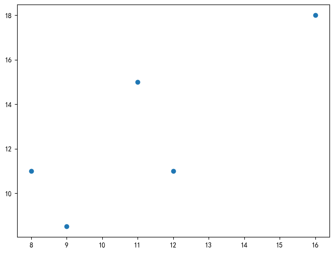
结论
训练后的模型用于新样本数据时,R^2为0.6620,模型欠拟合,以上新样本数据的散点图能够较好回答模型泛化能力弱的缘由
练习
收集某食品的商品尺寸、数量和价格,尝试用线性回归构建变量之间的关系。