Signal Filters Design Based on Digital Signal Processing-526互联

Thoeries

I. Fourier Series Expansion Algorithm

We can utilize the Fourier Series to produce the analog signal with some frequency components. For any signal, its Fourier series expansion is defined as

\[x(t) = \frac{A_0}{2}+\sum_{n=1}^{\infty}A_n\cos(n\Omega t+\varphi_n) \]

In the equation，$\frac{A_0}{2}$ represents the DC component, $A_1\cos(\Omega t+\varphi_1)$, represents the fundamental component of the signal, $A_n\cos(n\Omega t+\varphi_n)$ represents the nth harmonic component of the signal. Moreover, analog angular frequency $\Omega = \frac{2\pi}{T}=2\pi f$.
Therefore, in this project we select three different frequency components, that is $f_1, f_2, f_3$, to synthesize the final required analog signal:

\[x(t) = \frac{A_0}{2}+A_1\cos(2\pi f_1t+\varphi_1)+A_2\cos(2\times 2\pi f_2t+\varphi_2)+A_3\cos(3\times 2\pi f_3t+\varphi_3) \]

For simplicity, there we respectively select these values:

$A_0=0, A_1=1, A_2=1, A_3=1$ $$ \varphi_1=\varphi_2=\varphi_3=0 $$ Following above expression, we can get the generated analog signal: $$ x(t) = \cos(2\pi f_1t)+\cos(4\pi f_2t)+\cos(6\pi f_3t) $$

II. Sample the Analog Signal

Time Domain Sampling Theorem

According to the time domain sampling theorem, the sampling frequency must be greater than twice the signal cutoff frequency.
Let's assume that the sampling frequency is $F_s$, and the generated analog signal frequency satisfies: $F_1<F_2<F_3$, so the signal cutoff frequency is $F_c = F_3$. The sampling theorem is formally expressed as:

\[F_s > 2F_c \]

In this experiment，we respectively selected $F_1=10Hz, F_2=20Hz, F_3=30Hz$ to produce analog signal. So we can get the period and cutoff frequency of sampled signal:

\[T_c = \frac{1}{F_1}=0.1s, F_c = F_3 = 30Hz \]

Time-domain Window

For periodic continuous signals, we intercept at integer multiples of the period to obtain a sequence for spectrum analysis.

\[T_p=N*T_c, N\in Z^+ \]

Sampling Frequency

For a specific sampling frequency, we can get the sampling period $T_s$, and the number of sampling points $N$:

\[T_s = \frac{1}{F_s}, N=T_p*F_c \]

Therefore, we use sampling frequency of $F_s=90Hz, F_s=60Hz, F_s=40Hz$ to get time-domain signals.

Spectral Resolution

Spectral resolution is defined as the minimum separation between two signals of different frequencies:

\[\Delta f = \frac{F_s}{N}=\frac{1}{NT_s}=\frac{1}{T_p} \]

III. Spectral Analysis

In this section, we will analyse the Amplitude-Frequency Characteristics and Phase-Frequency Characteristics of the sampled signal.

Convert to Frequency

When analysing the spectral, we need to convert the $0\sim N-1$ to frequency sequence:

\[f_k = k*\frac{F_s}{N}, k=0,1,...N-1 \]

Convert to Real Amplitude

After we apply Discrete Fourier Transform to the sampled signal, the frequency-domain signal is complex-valued. And due to the time-domain signal is real-valued, the the frequency-domain signal is conjugate symmetric:

\[X(k) = X^*(N-k), k=0,1,...N-1 \]

For complex values, that means its real part is even symmetric about the middle point, and its imaginary part is odd symmetric about the middle point. This will be showed in the following figures.

Experiments

Experiment I: $T_p=3T_c, F_s=90$Hz

Samping Frequency $F_s = 3F_c(F_s > 2F_c)$
We use the sampling frequency of $F_s=90$Hz under the condition of $T_p=3T_c$.

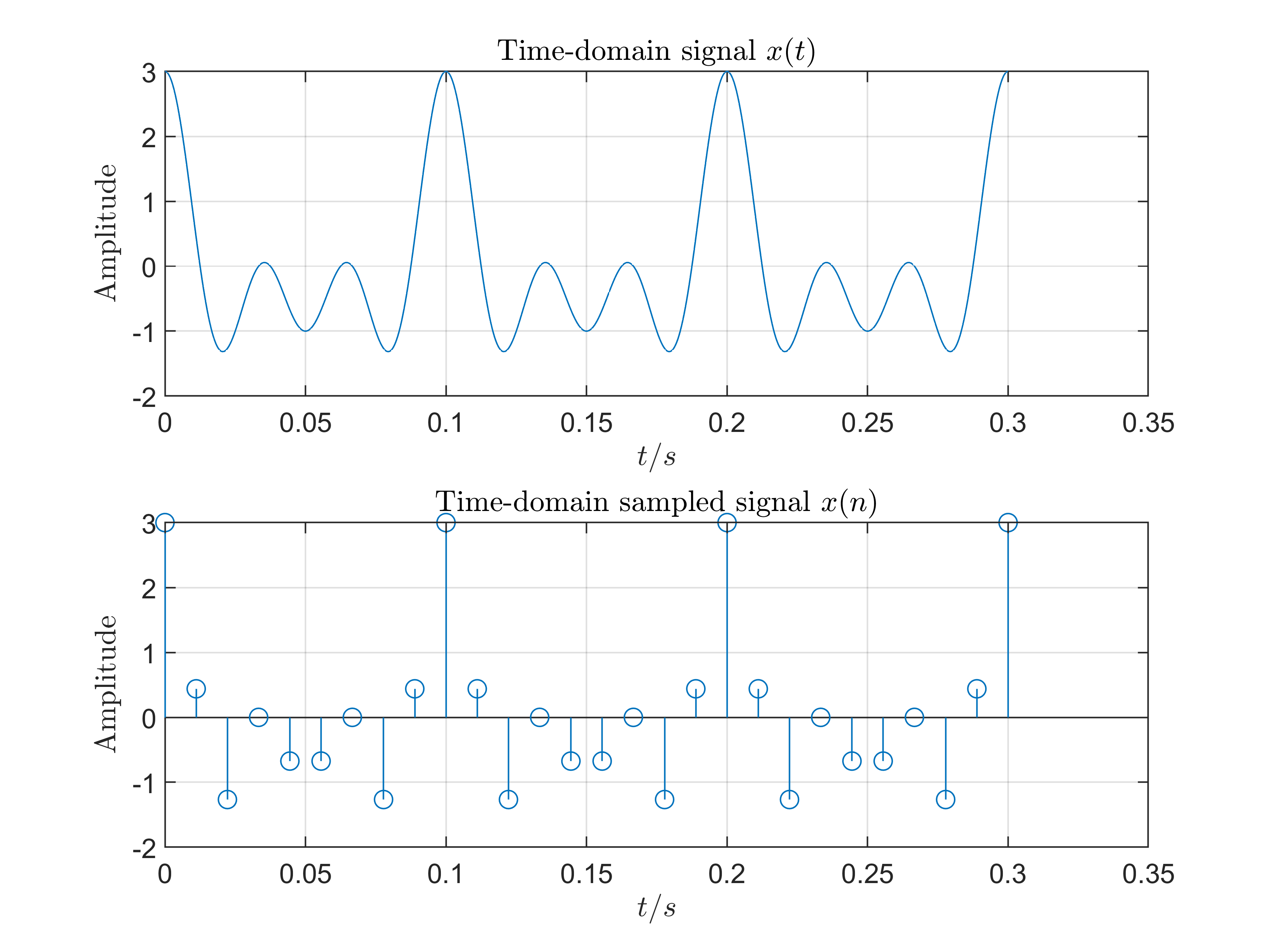
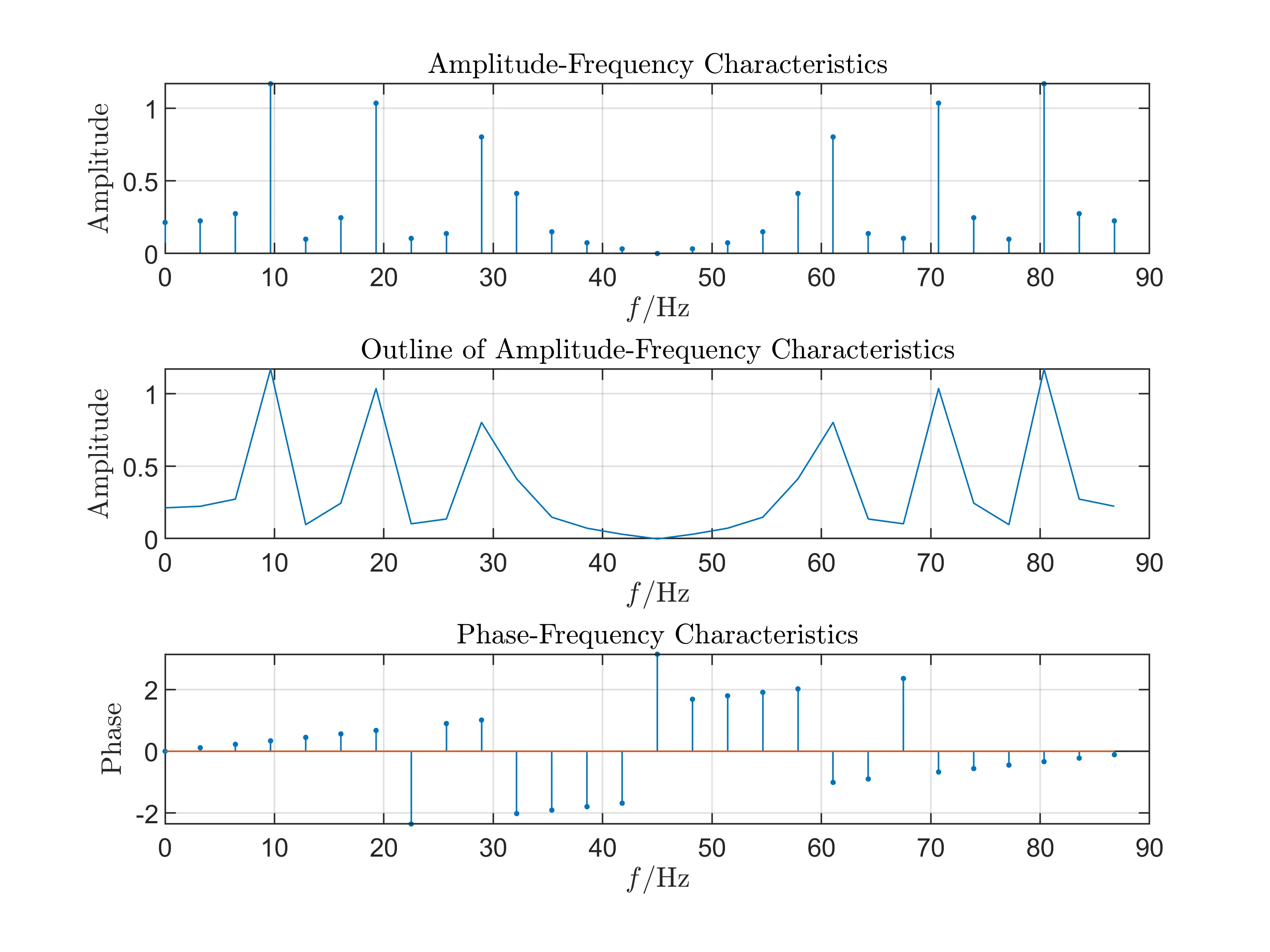
Conclusions
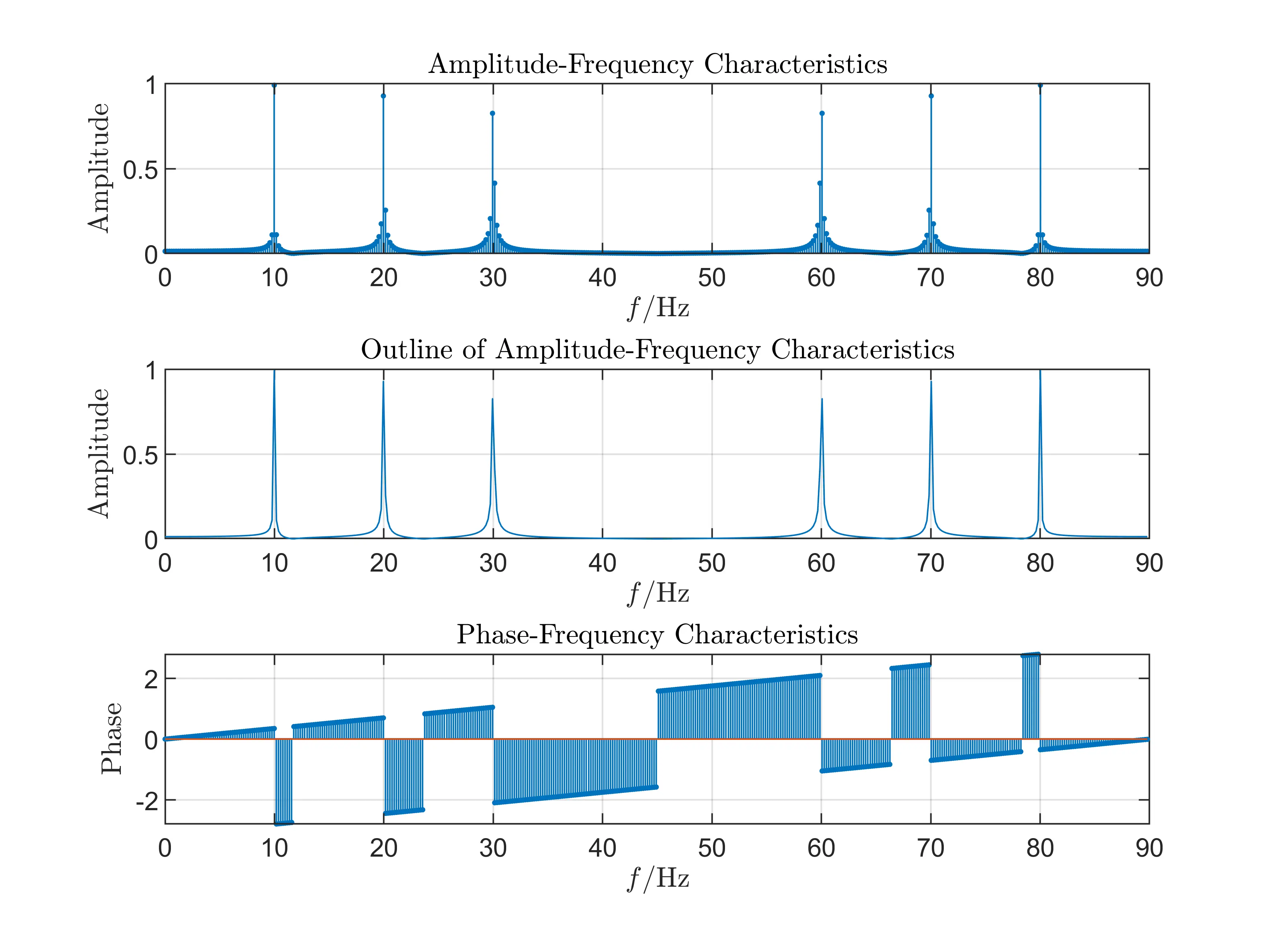
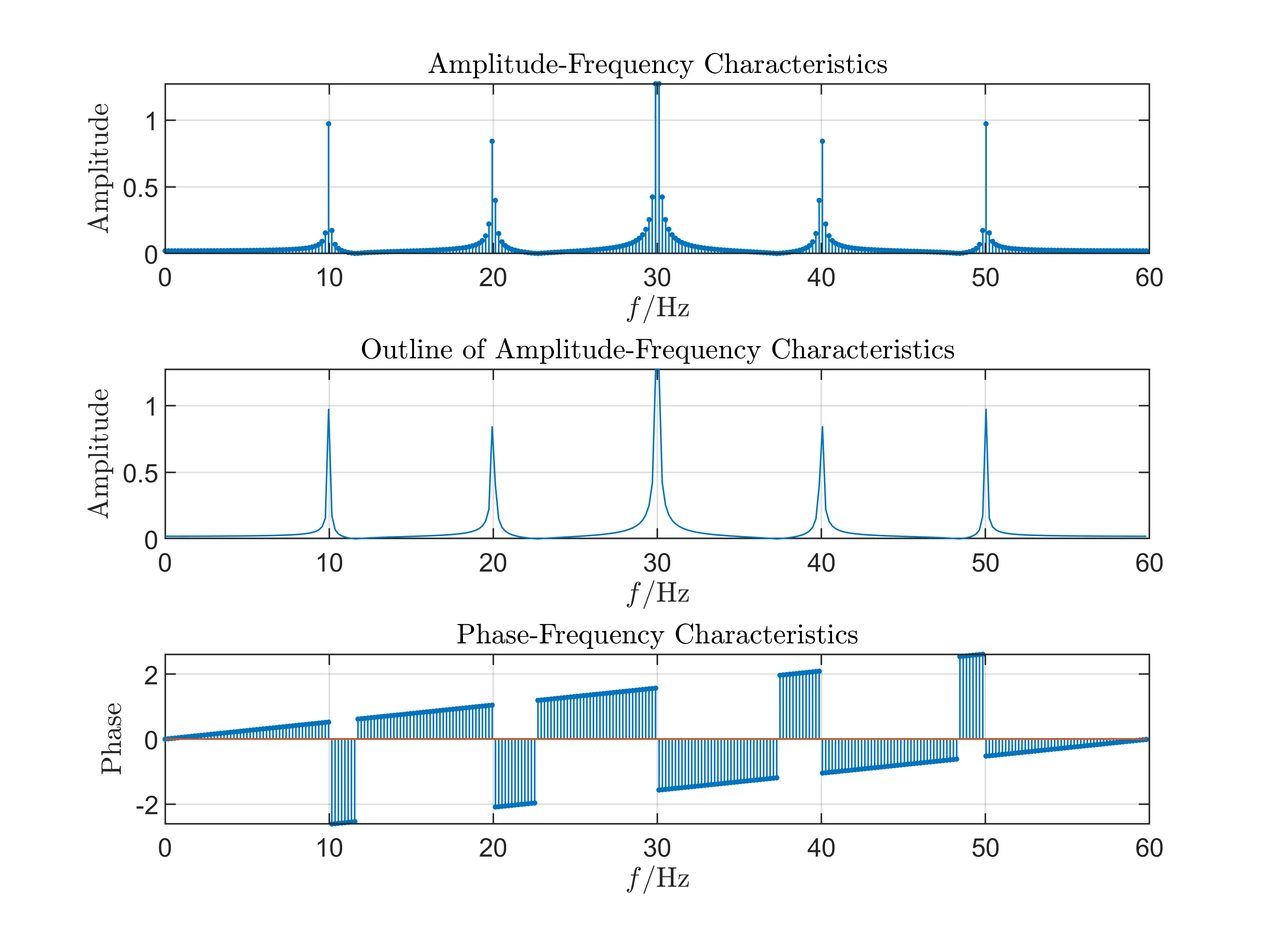
The sampling frequency satisfies the Time Domain Sampling Theorem so we can see there is no overlap in frequency domain about the amplitude-frequency characteristic. And when $f=10$Hz, $f=20$Hz, $f=30$Hz, we can get the amplitude very close to $1$ which is us defined in analop signal.

Experiment II: $T_p=3T_c, F_s=60$Hz

Samping Frequency $F_s = 2F_c(F_s = 2F_c)$
We use the sampling frequency of $F_s=60$Hz under the condition of $T_p=3T_c$.

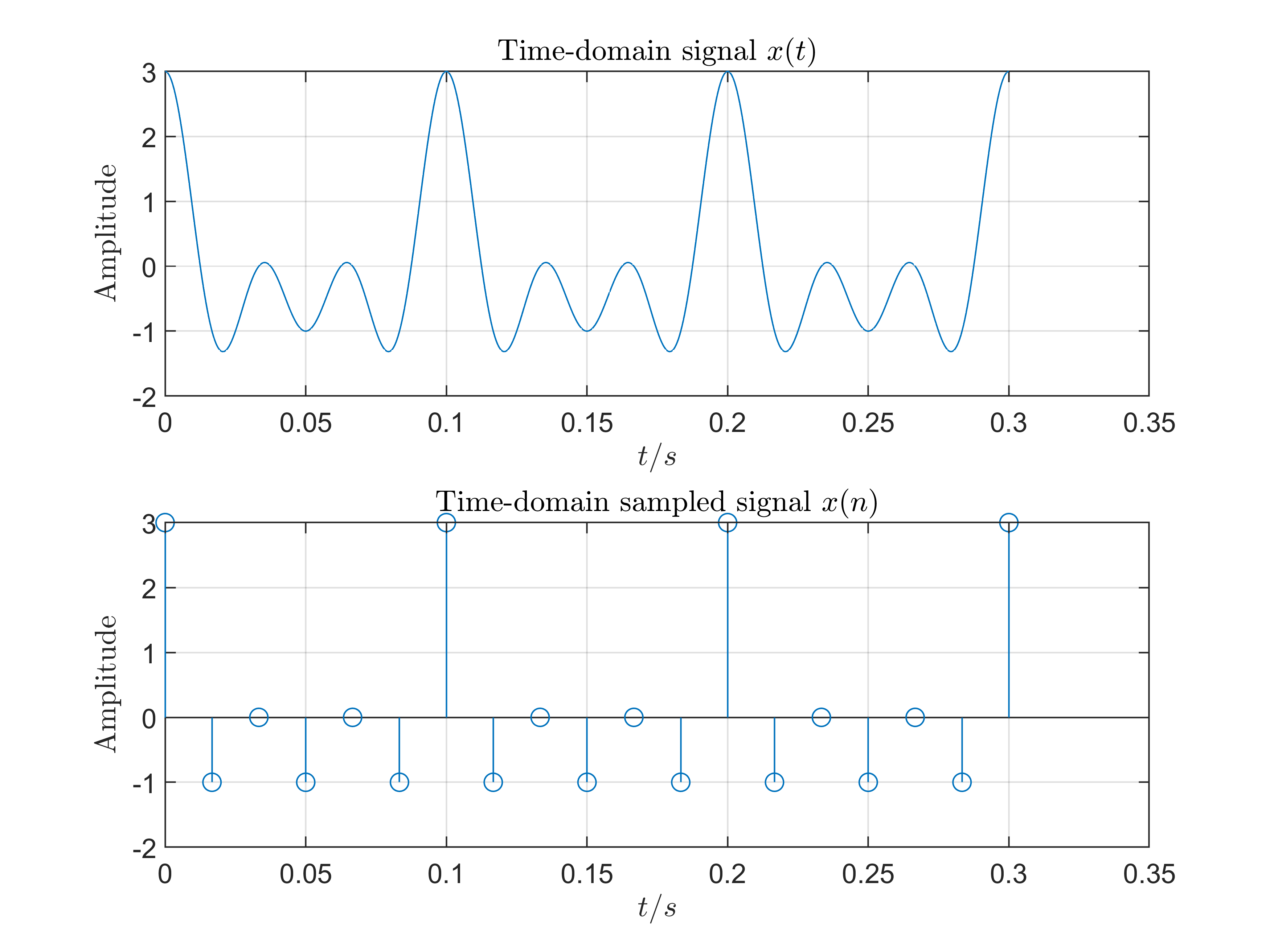
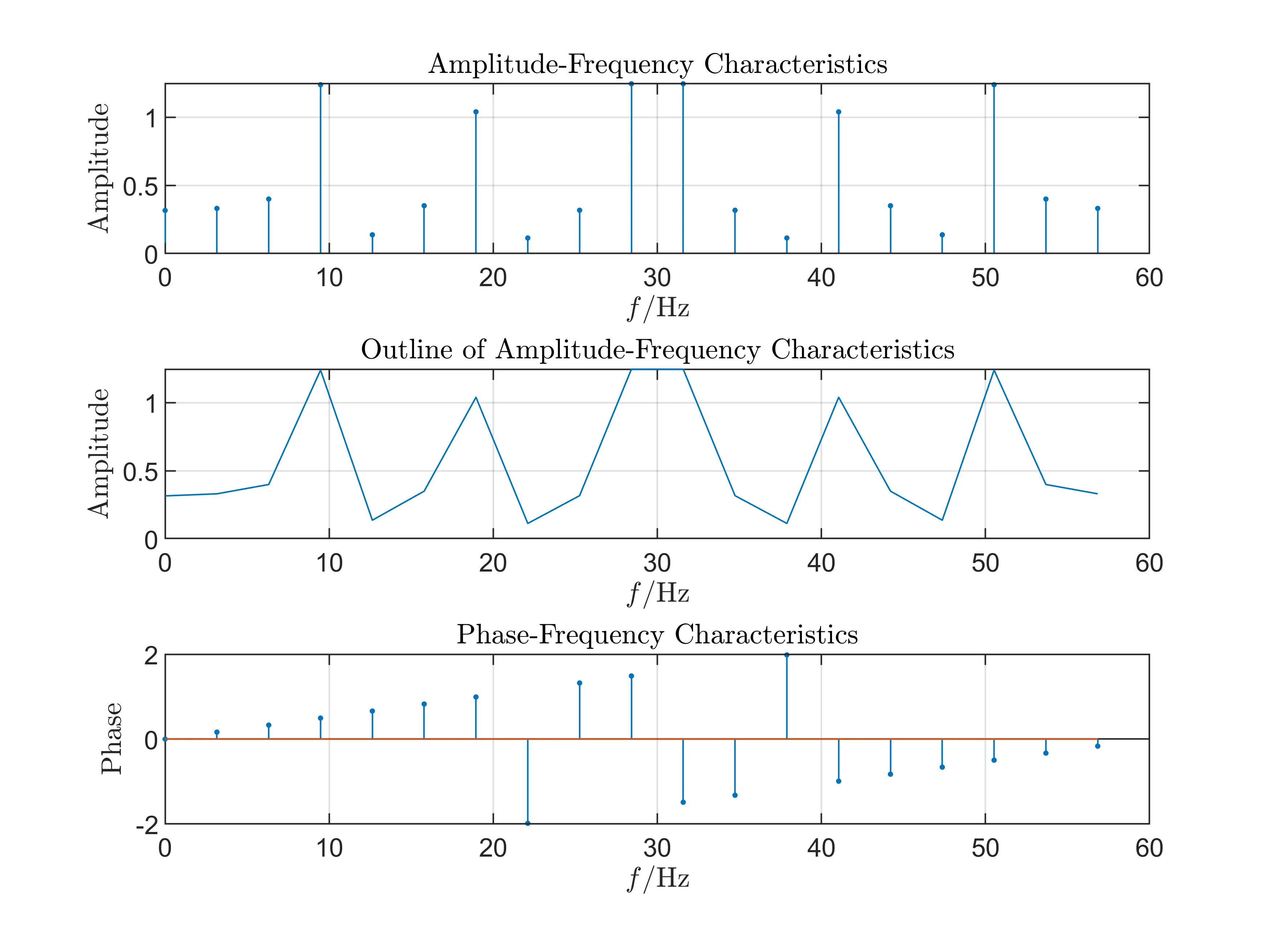
Conclusions
The sampling frequency equals the threhold of Time Domain Sampling Theorem so we can easily see that it will just become overlapping in frequency domain. And when $f=30$Hz that is also $F_s/2$ point, we can get this point very close to its symmetric frequency point.

Experiment III: $T_p=3T_c, F_s=40$Hz

Samping Frequency $F_s = \frac{4}{3}F_c(F_s < 2F_c)$
We use the sampling frequency of $F_s=40$Hz under the condition of $T_p=3T_c$.

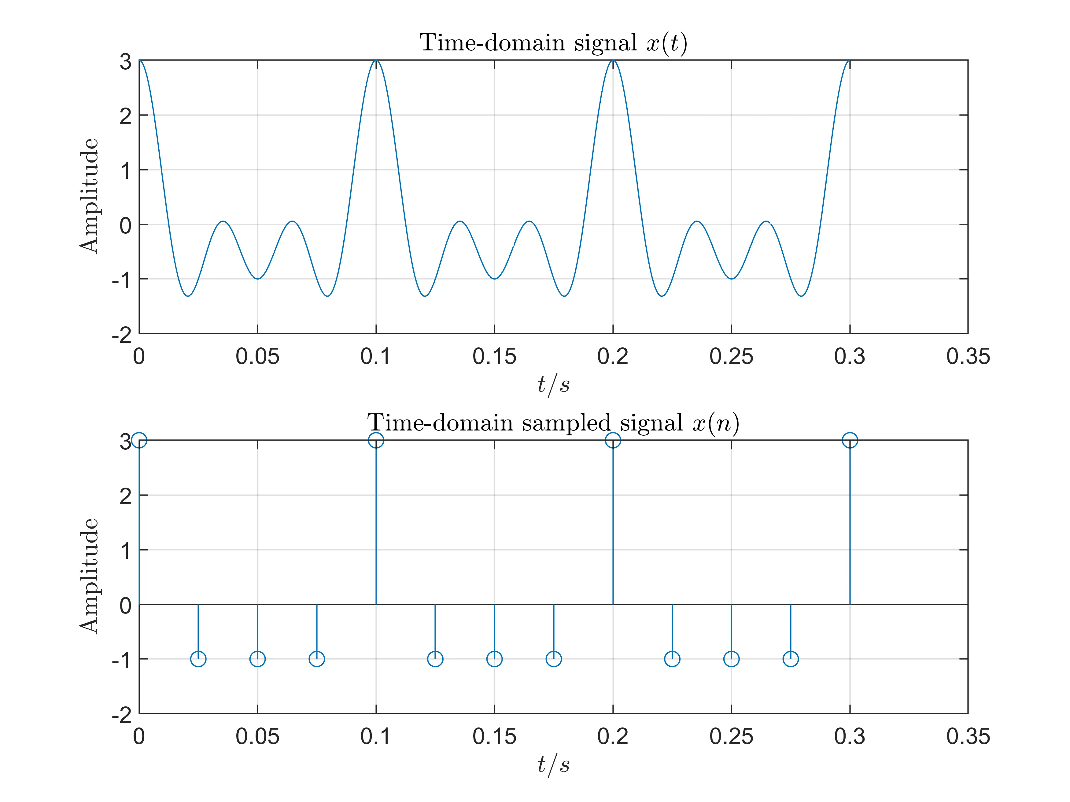
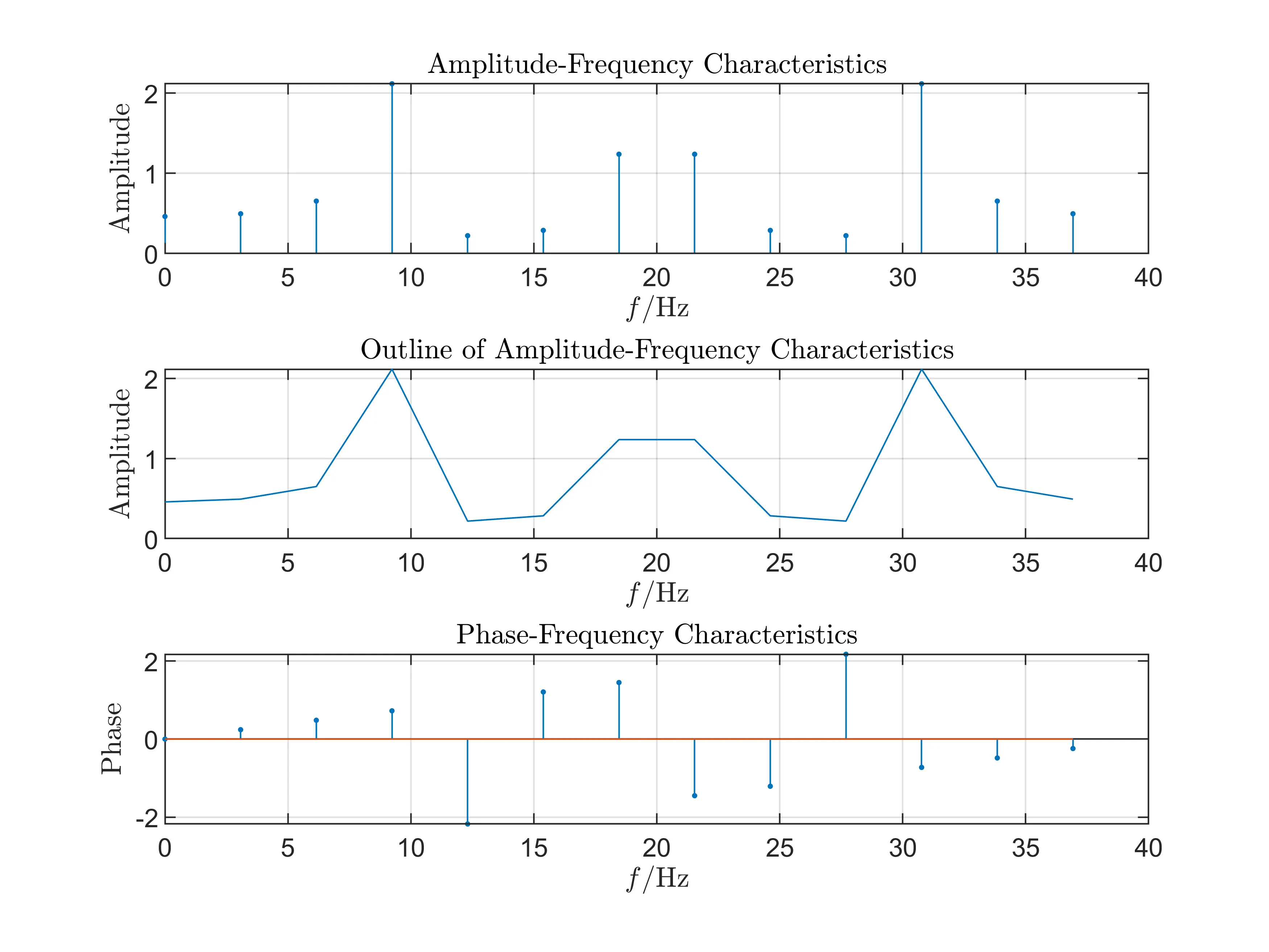
Conclusions
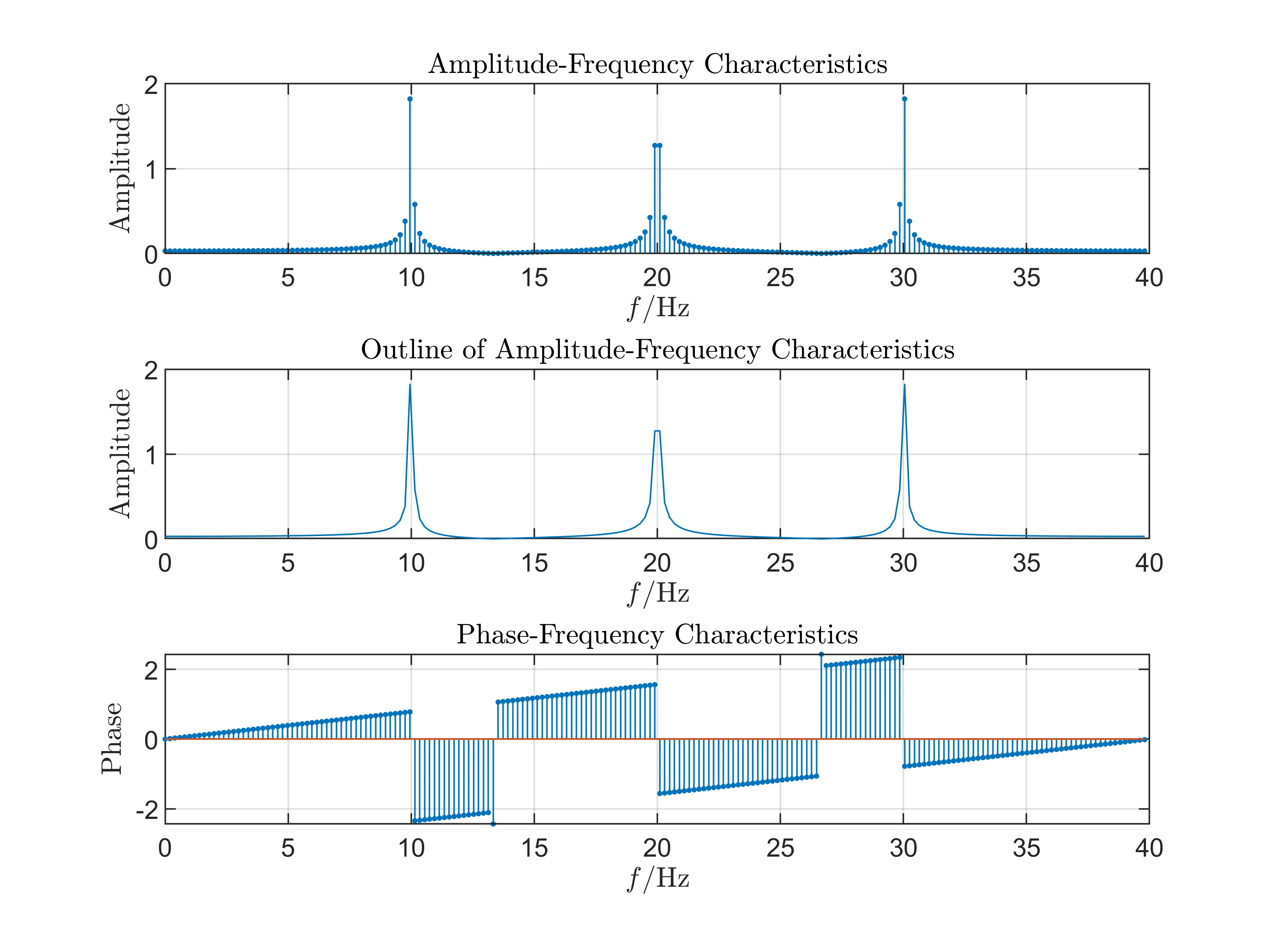
The sampling frequency do not equal the Time Domain Sampling Theorem so we can obviously see that it has discarded the third frequency $f=30$Hz, which is caused by overlapping in frequency domain.

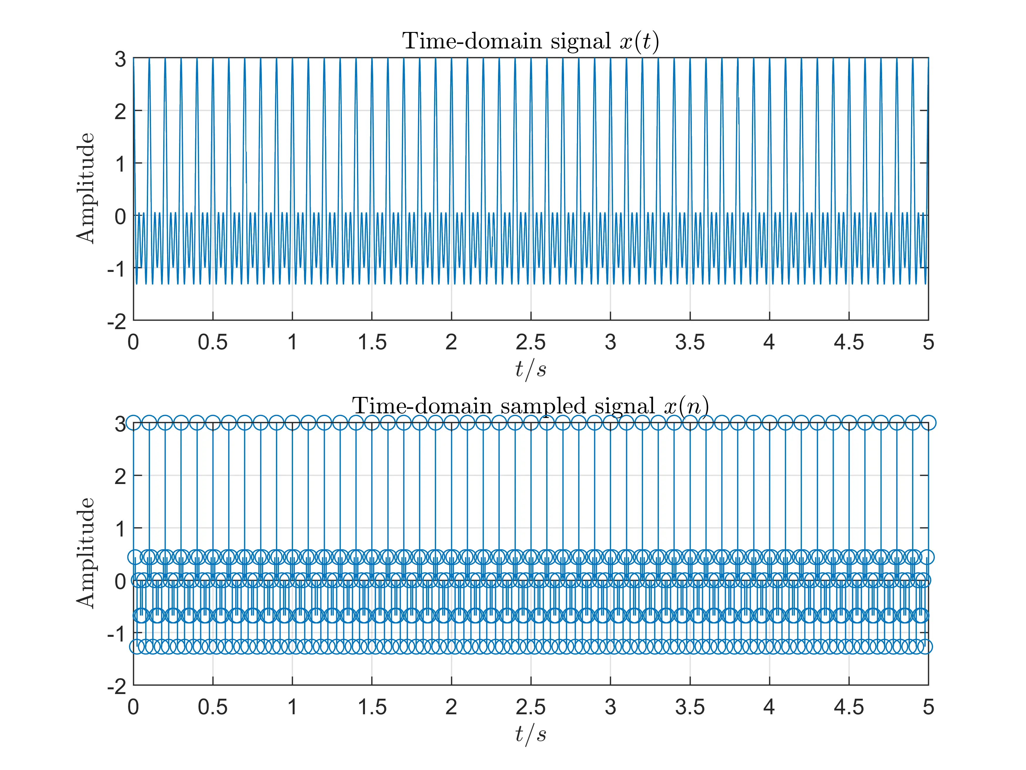
Note: in order to clearly analyse spectral of sampled signal, we also select the Time-domain Window of $T_p=50T_c$ to conduct experiments.

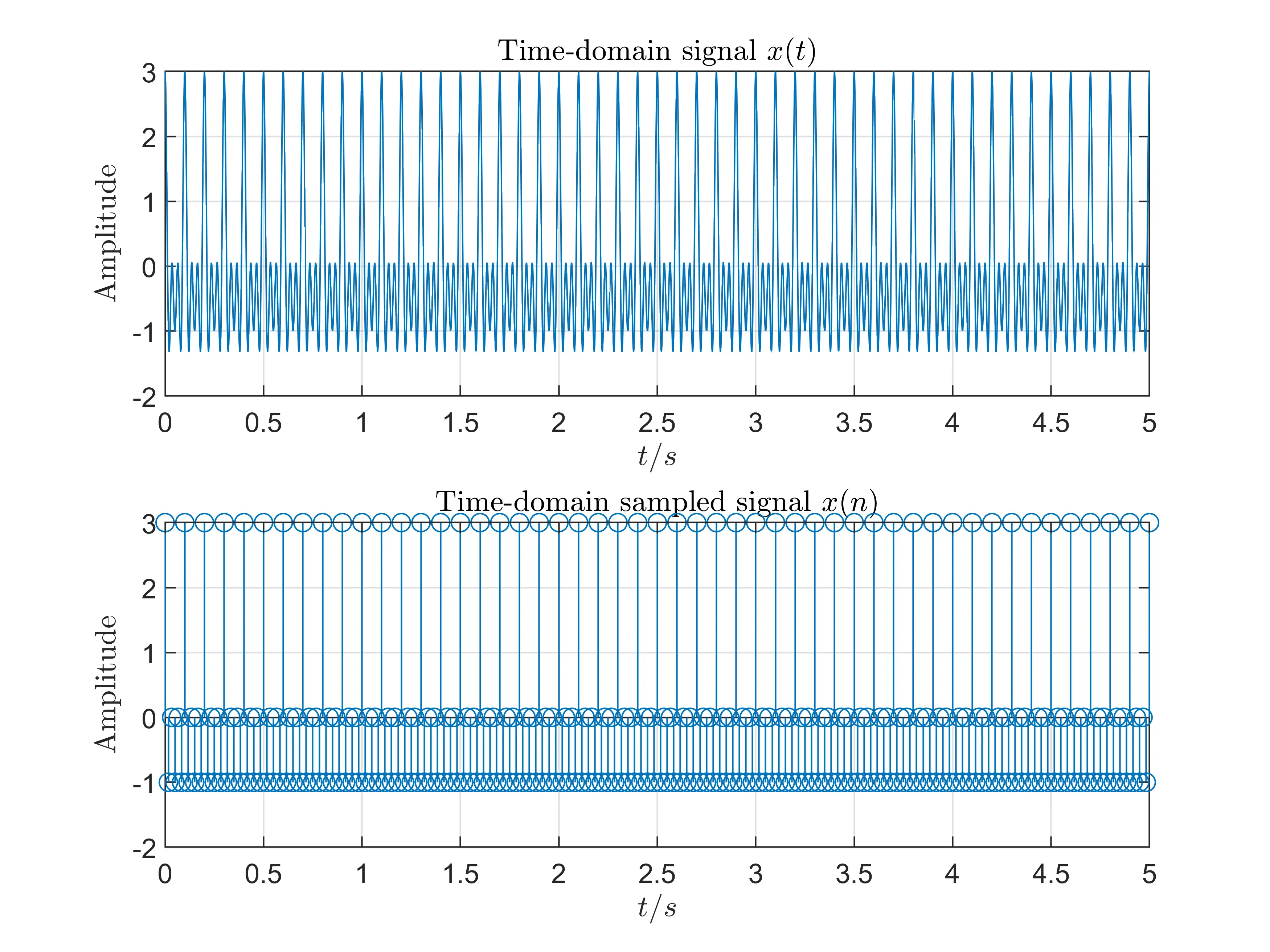
Experiment IV: $T_p=50T_c, F_s=90$Hz

Experiment V: $T_p=50T_c, F_s=60$Hz

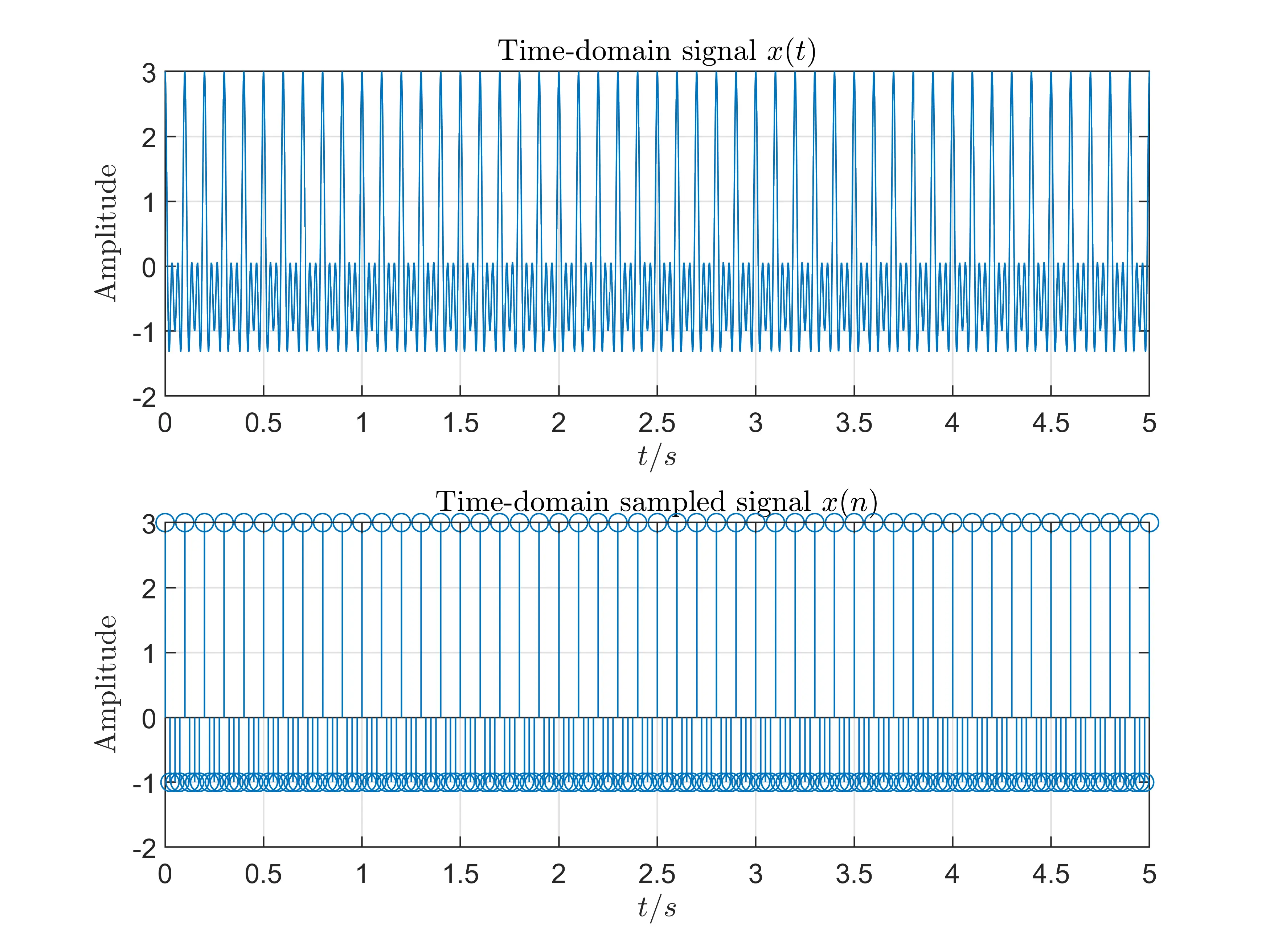
Experiment VI: $T_p=50T_c, F_s=40$Hz

Codes

%% Project Introdection:
%   This project is developed to design some signal filters based on digital
% signal processing.
clear, close all;
%% Produce and sample digital signal
f1 = 10;
f2 = 20;
f3 = 30;      % so the fc = f3 = 30Hz
Np = 3;      % number of periods for time-domain window
%% Experiment 1 (Choosing samling frequency fs = 3fc (fs > 2fs))
fs = 90;          % sampling frequency
xn1 = ProduceSamplingSignal(f1, f2, f3, fs, Np);
DFTAnalysis(xn1, fs);

%% Experiment 2 (Choosing samling frequency fs = 2fc)
fs = 60;          % sampling frequency
xn2 = ProduceSamplingSignal(f1, f2, f3, fs, Np);
DFTAnalysis(xn2, fs);

%% Experiment 3 (Choosing samling frequency fs < 2fc)
fs = 40;          % sampling frequency
xn3 = ProduceSamplingSignal(f1, f2, f3, fs, Np);
DFTAnalysis(xn3, fs);

function xn = ProduceSamplingSignal(f1, f2, f3, fs, Np)
% Function Description: 
%        We want to make a digital signal composed of three frequency
%        components and sample the produced signal.
% Inputs: 
%        f1, f2, f3: means our selected frequency components, fs
%            represents the sampling frequency.
%        Np: means the number of periods.
% Outputs:
%        xn: represents the sampled signal.

    period = 1/f1;        % the period of analog signal(assuming f1 is the minimal)
    T = Np*period;         % sampling time-domain window(several periods)
    Ts = 1 / fs;          % sampling timestep
    t0 = 0: Ts : T;       % samping sequence of discrete sampling points
    t = 0: 0.0001: T;     % analog time sequence

    % Step I: Produce digital signal
    xt = cos(2*pi*f1*t) + cos(2*pi*f2*t) + cos(2*pi*f3*t);
    % Step II: Sample produced signal
    xn = cos(2*pi*f1*t0) + cos(2*pi*f2*t0) + cos(2*pi*f3*t0);

    % Step III: Visualize produced signal and sampled signal
    figure;
    subplot(2, 1, 1);
    plot(t, xt);
    txt = title('Time-domain signal $x(t)$');
    set(txt, 'Interpreter', 'latex');
    txt = xlabel('$t/s$');
    set(txt, 'Interpreter', 'latex');
    txt = ylabel('Amplitude');
    set(txt, 'Interpreter', 'latex');
    grid on

    subplot(2, 1, 2);
    stem(t0, xn);
    txt = title('Time-domain sampled signal $x(n)$');
    set(txt, 'Interpreter', 'latex');
    txt = ylabel('Amplitude');
    set(txt, 'Interpreter', 'latex');
    txt = xlabel('$t/s$');
    set(txt, 'Interpreter', 'latex');
    grid on
end

function DFTAnalysis(xn, fs)
% Function Description:
%       This function calculates the DFT[x(n)] and do spectral analysis.
% Inputs:
%       xn: digital discrete signal
%       fs: sampling frequency
% Outputs:
%       No return

    N = length(xn);    % number of sampling points
    df = fs / N;       % spectral resolution
    f = (0:N-1)*df;    % tranverse to the frequncy sequence

    % DFT using FFT algorithm
    Xk = fft(xn, N);   
    % Tranverse to the real amplitude
    RM = 2*abs(Xk)/N;

    % Amplitude-Frequency Characteristics
    figure;
    subplot(3,1,1);
    stem(f, RM,'.');
    txt = title('Amplitude-Frequency Characteristics');
    set(txt, 'Interpreter', 'latex');
    txt = xlabel('$f$/Hz');
    set(txt, 'Interpreter', 'latex');
    txt = ylabel('Amplitude');
    set(txt, 'Interpreter', 'latex');
    grid on;

    % Outline of Amplitude-Frequency Characteristics
    subplot(3,1,2);
    plot(f, RM);
    txt = title('Outline of Amplitude-Frequency Characteristics');
    set(txt, 'Interpreter', 'latex');
    txt = xlabel('$f$/Hz');
    set(txt, 'Interpreter', 'latex');
    txt = ylabel('Amplitude');
    set(txt, 'Interpreter', 'latex');
    grid on;

    % Phase-Frequency Characteristics
    subplot(3,1,3);
    stem(f, angle(Xk),'.'); 
    line([(N-1)*df, 0],[0,0]);
    txt = title('Phase-Frequency Characteristics');
    set(txt, 'Interpreter', 'latex');
    txt = xlabel('$f$/Hz');
    set(txt, 'Interpreter', 'latex');
    txt = ylabel('Phase');
    set(txt, 'Interpreter', 'latex');
    grid on;
end