一.选题背景
驾驶员的疲劳和睡意是道路交通安全的重要隐患之一。据统计,疲劳驾驶导致的交通事故占比较高,甚至可能造成生命和财产的巨大损失。因此,开发一种有效的驾驶员睡意检测系统对于提高交通安全具有重要意义。
通过监测驾驶员的眼部数据等,可以建立一个机器学习模型来判断驾驶员是否处于疲劳或睡意状态。这样的模型可以实时监测驾驶员的状态,并在发现异常时提醒驾驶员或采取相应的措施,从而减少疲劳驾驶导致的交通事故风险。
二.机器学习案例设计方案
1.本题采用的测试集与训练集来源于网站www.kaggle.com
2.采用keras与sklearn框架进行机器学习,matplotlib绘制图形
3.一开始想使用keras工具进行ROC曲线、精确度-召回率曲线、计算混淆矩阵是系统报错,不知如何解决,后更换为用sklearn工具处理
三.机器学习的实现步骤
1.目的
提高交通安全:驾驶员的疲劳和睡意是道路交通事故的重要原因之一。通过训练一个有效的睡意检测模型,可以及时发现驾驶员的疲劳状态,提醒他们采取相应的措施,从而减少疲劳驾驶引起的交通事故风险,提高交通安全水平。
保护驾驶员健康:长时间的驾驶或夜间驾驶容易导致驾驶员疲劳和睡意,对他们的身体健康造成威胁。通过睡意检测模型,可以实时监测驾驶员的状态,并在发现疲劳或睡意迹象时提醒他们休息或采取其他必要的措施,保护驾驶员的健康。
2.数据
下载来的数据集已分好包裹,无需进行数据集与测试集的切分
3.初步分析特征工程
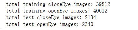
用代码访问文件夹,读取文件夹中图片的个数
import os
import pandas as pd
from keras.datasets import mnist
import keras
from keras import layers
from keras import models
import matplotlib.pyplot as plt
from keras.layers import Dense, Dropout, Activation, Flatten
from keras.utils import to_categorical
from keras import optimizers
from keras.preprocessing.image import ImageDataGenerator
from keras.models import load_model
from keras.preprocessing import image
import numpy as np
train_path="E:pythonmath/PreparedData/train/"
print('total training closeEye images:', len(os.listdir(train_path+"closeEye")))
print('total training openEye images:', len(os.listdir(train_path+"openEye")))
test_path="E:pythonmath/PreparedData/test/"
print('total test closeEye images:', len(os.listdir(test_path+"closeEye")))
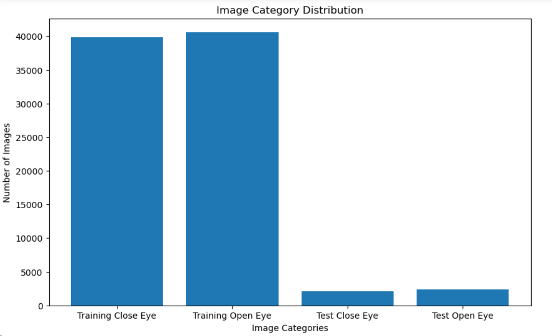
print('total test openEye images:', len(os.listdir(test_path+"openEye")))用可视化的方法可以直观的看到测试集与训练集的数据,这里采用比较合适的饼图、直方图与热力图展示


import matplotlib.pyplot as plt
import os
# 定义数据
train_path="E:pythonmath/PreparedData/train/"
test_path="E:pythonmath/PreparedData/test/"
training_closeEye_images = len(os.listdir(train_path + "closeEye"))
training_openEye_images = len(os.listdir(train_path + "openEye"))
test_closeEye_images = len(os.listdir(test_path + "closeEye"))
test_openEye_images = len(os.listdir(test_path + "openEye"))

# 定义标签
labels = ['Training Close Eye', 'Training Open Eye', 'Test Close Eye', 'Test Open Eye']
values = [training_closeEye_images, training_openEye_images, test_closeEye_images, test_openEye_images]
# 设置图形尺寸
plt.figure(figsize=(10, 6))
# 绘制柱状图
plt.bar(labels, values)
plt.xlabel('Image Categories')
plt.ylabel('Number of Images')
plt.title('Image Category Distribution')
plt.show()

# 定义标签
sizes = [training_closeEye_images, training_openEye_images, test_closeEye_images, test_openEye_images]
# 绘制饼图
plt.pie(sizes, labels=labels, autopct='%1.1f%%')
plt.title('Image Category Distribution')
# 设置图形为等比例圆形
plt.axis('equal')
# 显示图形
plt.show()
# 创建类别数量矩阵
data = np.array([[training_closeEye_images, training_openEye_images],
                 [test_closeEye_images, test_openEye_images]])
# 定义标签
labels = ['Close Eye', 'Open Eye']
categories = ['Training', 'Validation']
# 设置图形尺寸
plt.figure(figsize=(6, 4))
# 绘制热力图
heatmap = plt.imshow(data, cmap='hot')
# 添加数值标签
for i in range(len(categories)):
    for j in range(len(labels)):
        plt.text(j, i, data[i, j], ha='center', va='center', color='white')
# 设置坐标轴
plt.xticks(range(len(labels)), labels)
plt.yticks(range(len(categories)), categories)
# 添加颜色标尺
plt.colorbar(heatmap)
# 添加标题和标签
plt.title('Image Category Distribution')
plt.xlabel('Data Type')
plt.ylabel('Image Category')
# 显示图表
plt.show()
4.模型
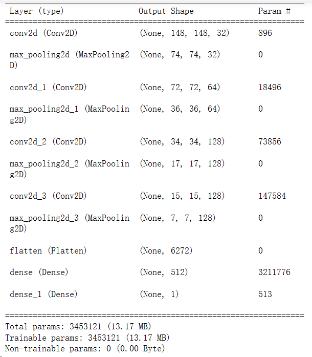
1.搭建卷积神经网络模型,让模型可以从原始数据中自动学习特征表示,并在睡意检测任务中表现出很好的性能。
model = models.Sequential()
#第一个卷积层作为输入层,32个3*3卷积核,输入形状input_shape = (150,150,3)
# 输出图片尺寸:150-3+1=148*148,参数数量:32*3*3*3+32=896
model.add(layers.Conv2D(32,(3,3),activation = 'relu',input_shape = (150,150,3)))
model.add(layers.MaxPooling2D((2,2)))# 输出图片尺寸:148/2=74*74
#输出图片尺寸:74-3+1=72*72,参数数量:64*3*3*32+64=18496
model.add(layers.Conv2D(64,(3,3),activation = 'relu'))
model.add(layers.MaxPooling2D((2,2)))# 输出图片尺寸:72/2=36*36
# 输出图片尺寸:36-3+1=34*34,参数数量:128*3*3*64+128=73856
model.add(layers.Conv2D(128,(3,3),activation = 'relu'))
model.add(layers.MaxPooling2D((2,2)))# 输出图片尺寸:34/2=17*17
model.add(layers.Conv2D(128,(3,3),activation = 'relu'))
model.add(layers.MaxPooling2D((2,2)))
model.add(layers.Flatten())
model.add(layers.Dense(512,activation = 'relu'))
model.add(layers.Dense(1,activation = 'sigmoid'))#sigmoid分类,输出是两类别
model.summary()
model.compile(loss='binary_crossentropy',
              optimizer=optimizers.RMSprop(lr=1e-4),
              metrics=['acc'])
2.存储层

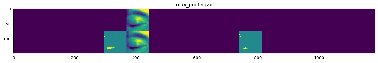

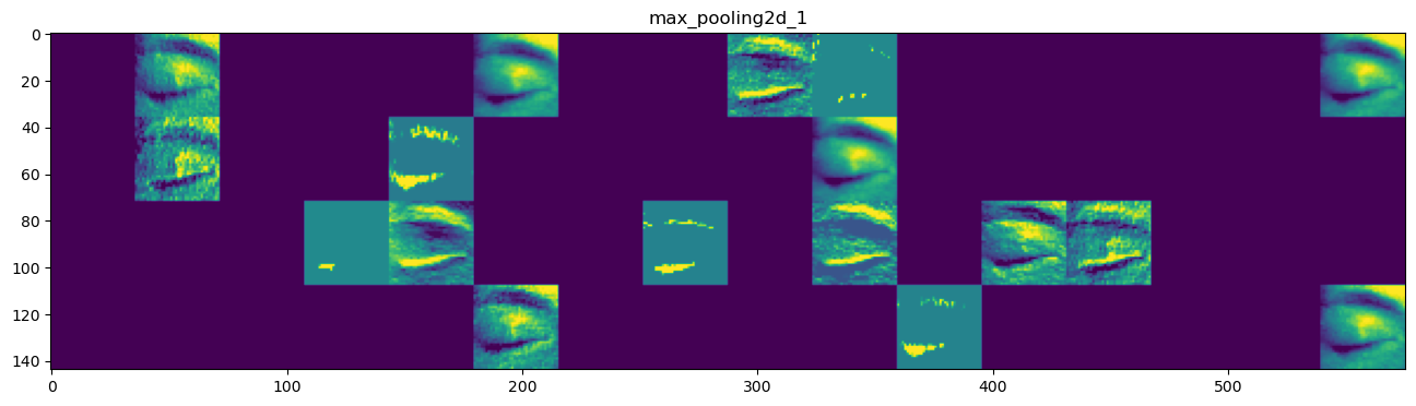
#存储层的名称
layer_names = []
for layer in model.layers[:4]:
    layer_names.append(layer.name)
# 每行显示16个特征图
images_pre_row = 16  #每行显示的特征图数
# 循环8次显示8层的全部特征图
for layer_name, layer_activation in zip(layer_names, activations):
    n_features = layer_activation.shape[-1] #保存当前层的特征图个数
    size = layer_activation.shape[1]  #保存当前层特征图的宽高
    n_col = n_features // images_pre_row #计算当前层显示多少行
    #生成显示图像的矩阵
    display_grid = np.zeros((size*n_col, images_pre_row*size))
    #遍历将每个特张图的数据写入到显示图像的矩阵中
    for col in range(n_col):
        for row in range(images_pre_row):
        	#保存该张特征图的矩阵(size,size,1)
            channel_image = layer_activation[0,:,:,col*images_pre_row+row]
            #为使图像显示更鲜明,作一些特征处理
            channel_image -= channel_image.mean()
            channel_image /= channel_image.std()
            channel_image *= 64
            channel_image += 128
            #把该特征图矩阵中不在0-255的元素值修改至0-255
            channel_image = np.clip(channel_image, 0, 255).astype("uint8")
            #该特征图矩阵填充至显示图像的矩阵中
            display_grid[col*size:(col+1)*size, row*size:(row+1)*size] = channel_image


    scale = 1./size
    #设置该层显示图像的宽高
    plt.figure(figsize=(scale*display_grid.shape[1],scale*display_grid.shape[0]))
    plt.title(layer_name)
    plt.grid(False)
    #显示图像
plt.imshow(display_grid, aspect="auto", cmap="viridis")5.设置必须参数
-
train_dir:训练集图片目录的路径。这应该是一个包含训练图像的文件夹的路径。 -
validation_dir:验证集图片目录的路径。这应该是一个包含验证图像的文件夹的路径。 -
target_size:输入训练图像的尺寸。在代码中设置为(150, 150),表示将输入图像调整为150x150的大小。 -
batch_size:每个训练批次中的图像数量。在代码中设置为20,表示每次训练模型时使用20个图像。 -
class_mode:分类模式。在代码中设置为'binary',表示进行二分类任务。
#归一化
import matplotlib.pyplot as plt
train_datagen = ImageDataGenerator(rescale = 1./255)
test_datagen = ImageDataGenerator(rescale = 1./255)
train_dir = 'E:pythonmath/PreparedData/train' #指向训练集图片目录路径
train_generator = train_datagen.flow_from_directory(
train_dir,
target_size = (150,150),# 输入训练图像尺寸
batch_size = 20,
class_mode = 'binary') #
validation_dir = 'E:pythonmath/PreparedData/validation' #指向验证集图片目录路径
validation_generator = test_datagen.flow_from_directory(
validation_dir,
target_size = (150,150),
batch_size = 20,
class_mode = 'binary')
for data_batch,labels_batch in train_generator:
print('data batch shape:',data_batch.shape)
print('data batch shape:',labels_batch.shape)
break #生成器不会停止,会循环生成这些批量,所以我们就循环生成一次批量
# 将标签转换为独热编码
#训练模型50轮次
history = model.fit(
train_generator,
steps_per_epoch = 100,
epochs = 50,
validation_data = validation_generator,
validation_steps = 50)
# 绘制训练和验证准确率曲线
acc = history.history['acc']
val_acc = history.history['val_acc']
epochs = range(1, len(acc) + 1)
plt.plot(epochs, acc, 'bo', label='Training acc')
plt.plot(epochs, val_acc, 'b', label='Validation acc')
plt.title('Training and Validation Accuracy')
plt.xlabel('Epochs')
plt.ylabel('Accuracy')
plt.legend()
plt.figure()
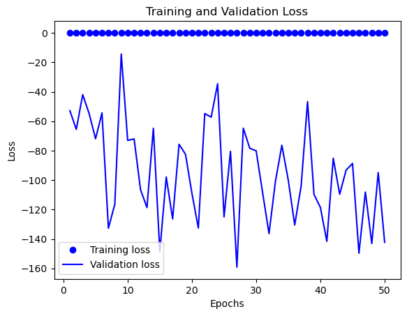
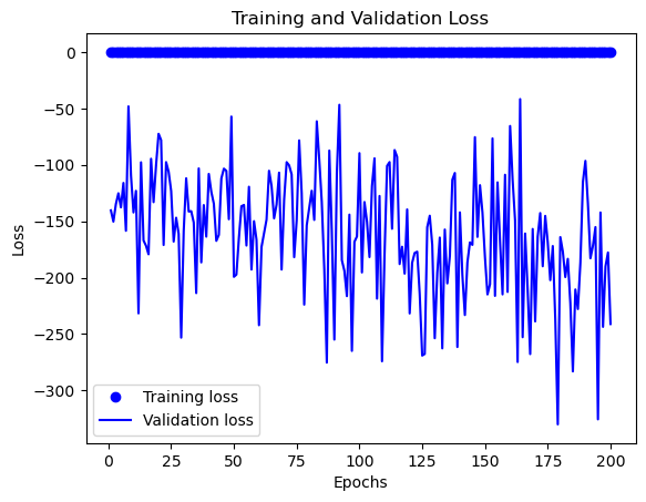
# 绘制训练和验证损失曲线
loss = history.history['loss']
val_loss = history.history['val_loss']
plt.plot(epochs, loss, 'bo', label='Training loss')
plt.plot(epochs, val_loss, 'b', label='Validation loss')
plt.title('Training and Validation Loss')
plt.xlabel('Epochs')
plt.ylabel('Loss')
plt.legend()
plt.show()
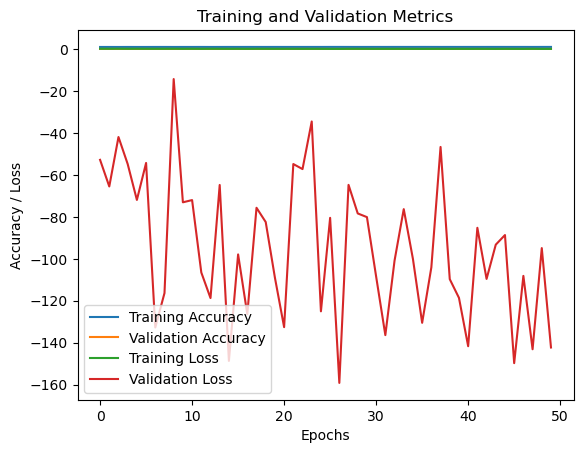
# 绘制训练和验证曲线
plt.plot(history.history['acc'], label='Training Accuracy')
plt.plot(history.history['val_acc'], label='Validation Accuracy')
plt.plot(history.history['loss'], label='Training Loss')
plt.plot(history.history['val_loss'], label='Validation Loss')
plt.xlabel('Epochs')
plt.ylabel('Accuracy / Loss')
plt.title('Training and Validation Metrics')
plt.legend()
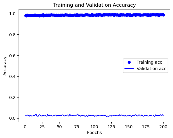
plt.show()在训练完后,在利用工具可视化训练和验证准确率曲线、训练和验证损失曲线、训练和验证曲线,这样能直观的看到训练过程中各种指标数据的变化

6.预测
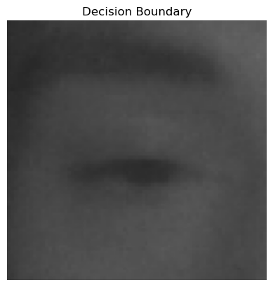
1.进行预测,绘制决策边界图
# 加载模型
model = load_model('E:pythonmath/PreparedData/eyes200.h5')
# 加载测试图像
img_path = "E:pythonmath/PreparedData/new_you.png"
img = image.load_img(img_path, target_size=(150, 150))
img_tensor = image.img_to_array(img) / 255.0
img_tensor = np.expand_dims(img_tensor, axis=0)
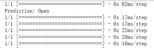
# 进行预测
result = model.predict(img_tensor)
prediction = "Open" if result > 0.5 else "Closed"
print("Prediction:", prediction)
# 绘制决策边界图
fig, ax = plt.subplots()
# 绘制关闭眼睛的决策边界
closed_eye_path = "E:pythonmath/PreparedData/test/closeEye/"
closed_eye_images = os.listdir(closed_eye_path)
for image_name in closed_eye_images:
image_path = os.path.join(closed_eye_path, image_name)
img = image.load_img(image_path, target_size=(150, 150))
img_array = image.img_to_array(img) / 255.0
prediction = model.predict(np.expand_dims(img_array, axis=0))
if prediction > 0.5:
ax.imshow(img_array)
break
# 绘制睁开眼睛的决策边界
open_eye_path = "E:pythonmath/PreparedData/test/openEye/"
open_eye_images = os.listdir(open_eye_path)
for image_name in open_eye_images:
image_path = os.path.join(open_eye_path, image_name)
img = image.load_img(image_path, target_size=(150, 150))
img_array = image.img_to_array(img) / 255.0
prediction = model.predict(np.expand_dims(img_array, axis=0))
if prediction <= 0.5:
ax.imshow(img_array)
break
plt.title("Decision Boundary")
plt.axis("off")
plt.show()2.使用模型进行预测,并获取预测结果的概率
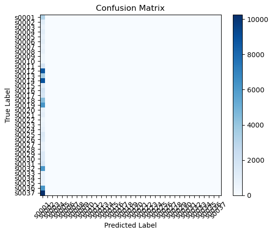
利用可视化图形工具绘制ROC曲线、精确度-召回率曲线、计算混淆矩阵


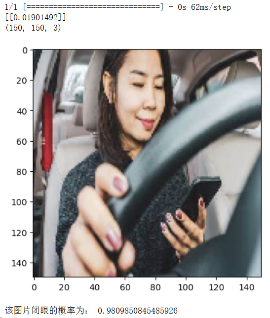
7.测试训练后的模型
这是使用进行50次训练后的模型识别的结果,判断图片中的人眼睛睁开的概率为约为0.628,考虑到图片的背景比较丰富,且隔着玻璃板,眼睛的区域比较模糊,这个结果还算是合理。

不过我还是想做尝试,然后我将训练次数提升至了200次


这是利用训练200次后的模型识别的结果
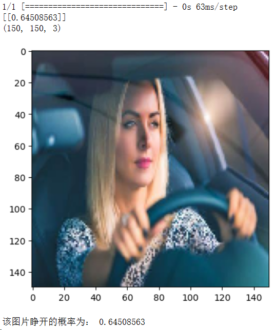
对睁眼图片的从判断0.628提升至0.645,识别的功能还是有明显的提升的
对闭眼图片的识别率是很高的,即使在图片背景较为丰富的且眼睛的区块也较小的情况下,也能清楚的识别
from keras.models import load_model
from keras.preprocessing import image
import matplotlib.pyplot as plt
import numpy as np

model = load_model('E:pythonmath/PreparedData/eyes.h5')

img_path = "E:pythonmath/PreparedData/you.png"
img = image.load_img(img_path, target_size=(150, 150))
img_tensor = image.img_to_array(img)
img_tensor = np.expand_dims(img_tensor, axis=0)
img_tensor /= 255.0

result = model.predict(img_tensor)
print(result)

img_scale = img_tensor[0]
print(img_scale.shape)

plt.imshow(img_scale)
plt.show()

if result[0][0] > 0.5:
    print('该图片睁开的概率为:', result[0][0])
else:
    print('该图片闭眼的概率为:', 1 - result[0][0])
import os
import pandas as pd
from keras.datasets import mnist
import keras
from keras import layers
from keras import models
import matplotlib.pyplot as plt
from keras.layers import Dense, Dropout, Activation, Flatten
from keras.utils import to_categorical
from keras import optimizers
from keras.preprocessing.image import ImageDataGenerator
from keras.models import load_model
from keras.preprocessing import image
import numpy as np
from sklearn.metrics import roc_curve, auc, precision_recall_curve, confusion_matrix
from sklearn.preprocessing import label_binarize
from PIL import Image

train_path="E:pythonmath/PreparedData/train/"
print('total training closeEye images:', len(os.listdir(train_path+"closeEye")))
print('total training openEye images:', len(os.listdir(train_path+"openEye")))
test_path="E:pythonmath/PreparedData/test/"
print('total test closeEye images:', len(os.listdir(test_path+"closeEye")))
print('total test openEye images:', len(os.listdir(test_path+"openEye")))
# 定义数据
train_path="E:pythonmath/PreparedData/train/"
test_path="E:pythonmath/PreparedData/test/"
training_closeEye_images = len(os.listdir(train_path + "closeEye"))
training_openEye_images = len(os.listdir(train_path + "openEye"))
test_closeEye_images = len(os.listdir(test_path + "closeEye"))
test_openEye_images = len(os.listdir(test_path + "openEye"))
# 定义标签
labels = ['Training Close Eye', 'Training Open Eye', 'Test Close Eye', 'Test Open Eye']
values = [training_closeEye_images, training_openEye_images, test_closeEye_images, test_openEye_images]
# 设置图形尺寸
plt.figure(figsize=(10, 6))
# 绘制柱状图
plt.bar(labels, values)
plt.xlabel('Image Categories')
plt.ylabel('Number of Images')
plt.title('Image Category Distribution')
plt.show()
# 定义标签
sizes = [training_closeEye_images, training_openEye_images, test_closeEye_images, test_openEye_images]
# 绘制饼图
plt.pie(sizes, labels=labels, autopct='%1.1f%%')
plt.title('Image Category Distribution')
# 设置图形为等比例圆形
plt.axis('equal')
# 显示图形
plt.show()
# 创建类别数量矩阵
data = np.array([[training_closeEye_images, training_openEye_images],
                 [test_closeEye_images, test_openEye_images]])
# 定义标签
labels = ['Close Eye', 'Open Eye']
categories = ['Training', 'Validation']
# 设置图形尺寸
plt.figure(figsize=(6, 4))
# 绘制热力图
heatmap = plt.imshow(data, cmap='hot')
# 添加数值标签
for i in range(len(categories)):
    for j in range(len(labels)):
        plt.text(j, i, data[i, j], ha='center', va='center', color='white')
# 设置坐标轴
plt.xticks(range(len(labels)), labels)
plt.yticks(range(len(categories)), categories)
# 添加颜色标尺
plt.colorbar(heatmap)
# 添加标题和标签
plt.title('Image Category Distribution')
plt.xlabel('Data Type')
plt.ylabel('Image Category')
# 显示图表
plt.show()
model = models.Sequential()
#第一个卷积层作为输入层,32个3*3卷积核,输入形状input_shape = (150,150,3)
# 输出图片尺寸:150-3+1=148*148,参数数量:32*3*3*3+32=896
model.add(layers.Conv2D(32,(3,3),activation = 'relu',input_shape = (150,150,3)))
model.add(layers.MaxPooling2D((2,2)))# 输出图片尺寸:148/2=74*74
#输出图片尺寸:74-3+1=72*72,参数数量:64*3*3*32+64=18496
model.add(layers.Conv2D(64,(3,3),activation = 'relu'))
model.add(layers.MaxPooling2D((2,2)))# 输出图片尺寸:72/2=36*36
# 输出图片尺寸:36-3+1=34*34,参数数量:128*3*3*64+128=73856
model.add(layers.Conv2D(128,(3,3),activation = 'relu'))
model.add(layers.MaxPooling2D((2,2)))# 输出图片尺寸:34/2=17*17
model.add(layers.Conv2D(128,(3,3),activation = 'relu'))
model.add(layers.MaxPooling2D((2,2)))
model.add(layers.Flatten())
model.add(layers.Dense(512,activation = 'relu'))
model.add(layers.Dense(1,activation = 'sigmoid'))#sigmoid分类,输出是两类别
model.summary()
model.compile(loss='binary_crossentropy',
              optimizer=optimizers.RMSprop(lr=1e-4),
              metrics=['acc'])
#归一化
train_datagen = ImageDataGenerator(rescale = 1./255)
test_datagen = ImageDataGenerator(rescale = 1./255)
train_dir = 'E:pythonmath/PreparedData/train'     #指向训练集图片目录路径
train_generator = train_datagen.flow_from_directory(
    train_dir,
    target_size = (150,150),#  输入训练图像尺寸
    batch_size = 20,
    class_mode = 'binary')  #
validation_dir = 'E:pythonmath/PreparedData/validation'  #指向验证集图片目录路径
validation_generator = test_datagen.flow_from_directory(
    validation_dir,
    target_size = (150,150),
    batch_size = 20,
    class_mode = 'binary')
for data_batch,labels_batch in train_generator:
    print('data batch shape:',data_batch.shape)
    print('data batch shape:',labels_batch.shape)
    break #生成器不会停止,会循环生成这些批量,所以我们就循环生成一次批量
# 将标签转换为独热编码
#训练模型200轮次
history = model.fit(
                    train_generator,
                    steps_per_epoch = 100,
                    epochs = 200,
                    validation_data = validation_generator,
                    validation_steps = 50)
# 绘制训练和验证准确率曲线
acc = history.history['acc']
val_acc = history.history['val_acc']
epochs = range(1, len(acc) + 1)
plt.plot(epochs, acc, 'bo', label='Training acc')
plt.plot(epochs, val_acc, 'b', label='Validation acc')
plt.title('Training and Validation Accuracy')
plt.xlabel('Epochs')
plt.ylabel('Accuracy')
plt.legend()
plt.figure()
# 绘制训练和验证损失曲线
loss = history.history['loss']
val_loss = history.history['val_loss']
plt.plot(epochs, loss, 'bo', label='Training loss')
plt.plot(epochs, val_loss, 'b', label='Validation loss')
plt.title('Training and Validation Loss')
plt.xlabel('Epochs')
plt.ylabel('Loss')
plt.legend()
plt.show()
# 绘制训练和验证曲线
plt.plot(history.history['acc'], label='Training Accuracy')
plt.plot(history.history['val_acc'], label='Validation Accuracy')
plt.plot(history.history['loss'], label='Training Loss')
plt.plot(history.history['val_loss'], label='Validation Loss')
plt.xlabel('Epochs')
plt.ylabel('Accuracy / Loss')
plt.title('Training and Validation Metrics')
plt.legend()
plt.show()
model.save('E:pythonmath/PreparedData/eyes200.h5')
model = load_model('E:pythonmath/PreparedData/eyes200.h5')
#从测试集中读取一条样本
img_path = "E:pythonmath/PreparedData/train/closeEye/s0002_00294_0_0_0_0_1_01.png"
img = image.load_img(img_path, target_size=(150,150))
img_tensor = image.img_to_array(img)
img_tensor = np.expand_dims(img_tensor, axis=0)
img_tensor /= 255.
print(img_tensor.shape)
#显示样本
plt.imshow(img_tensor[0])
plt.show()
layer_outputs = [layer.output for layer in model.layers[:8]]
activation_model = models.Model(inputs=model.input, outputs=layer_outputs)
#获得改样本的特征图
activations = activation_model.predict(img_tensor)
#显示第一层激活输出特的第一个滤波器的特征图
first_layer_activation = activations[0]
plt.matshow(first_layer_activation[0,:,:,1],  cmap="viridis")
#存储层的名称
layer_names = []
for layer in model.layers[:4]:
    layer_names.append(layer.name)
# 每行显示16个特征图
images_pre_row = 16  #每行显示的特征图数
# 循环8次显示8层的全部特征图
for layer_name, layer_activation in zip(layer_names, activations):
    n_features = layer_activation.shape[-1] #保存当前层的特征图个数
    size = layer_activation.shape[1]  #保存当前层特征图的宽高
    n_col = n_features // images_pre_row #计算当前层显示多少行
    #生成显示图像的矩阵
    display_grid = np.zeros((size*n_col, images_pre_row*size))
    #遍历将每个特张图的数据写入到显示图像的矩阵中
    for col in range(n_col):
        for row in range(images_pre_row):
        	#保存该张特征图的矩阵(size,size,1)
            channel_image = layer_activation[0,:,:,col*images_pre_row+row]
            #为使图像显示更鲜明,作一些特征处理
            channel_image -= channel_image.mean()
            channel_image /= channel_image.std()
            channel_image *= 64
            channel_image += 128
            #把该特征图矩阵中不在0-255的元素值修改至0-255
            channel_image = np.clip(channel_image, 0, 255).astype("uint8")
            #该特征图矩阵填充至显示图像的矩阵中
            display_grid[col*size:(col+1)*size, row*size:(row+1)*size] = channel_image
    scale = 1./size
    #设置该层显示图像的宽高
    plt.figure(figsize=(scale*display_grid.shape[1],scale*display_grid.shape[0]))
    plt.title(layer_name)
    plt.grid(False)
    #显示图像
    plt.imshow(display_grid, aspect="auto", cmap="viridis")
validation_generator.reset()
# 使用模型进行预测,并获取预测结果的概率
predicted_probs = model.predict(validation_generator)
num_classes = predicted_probs.shape[1]
# 获取真实标签
true_labels = validation_generator.classes
# 将真实标签进行二值化处理
true_labels_binary = label_binarize(true_labels, classes=range(num_classes))
# 绘制ROC曲线
fpr = dict()
tpr = dict()
roc_auc = dict()
for i in range(num_classes):
    fpr[i], tpr[i], _ = roc_curve(true_labels_binary[:, i], predicted_probs[:, i])
    roc_auc[i] = auc(fpr[i], tpr[i])
plt.figure()
for i in range(num_classes):
    plt.plot(fpr[i], tpr[i], label='ROC curve (area = %0.2f)' % roc_auc[i])
plt.plot([0, 1], [0, 1], 'k--')
plt.xlim([0.0, 1.0])
plt.ylim([0.0, 1.05])
plt.xlabel('False Positive Rate')
plt.ylabel('True Positive Rate')
plt.title('Receiver Operating Characteristic')
plt.legend(loc="lower right")
plt.show()
# 绘制精确度-召回率曲线
precision = dict()
recall = dict()
for i in range(num_classes):
    precision[i], recall[i], _ = precision_recall_curve(true_labels_binary[:, i], predicted_probs[:, i])
plt.figure()
for i in range(num_classes):
    plt.plot(recall[i], precision[i], label='Precision-Recall curve')
plt.xlabel('Recall')
plt.ylabel('Precision')
plt.title('Precision-Recall Curve')
plt.legend(loc="lower right")
plt.show()
# 计算混淆矩阵
predicted_labels = np.argmax(predicted_probs, axis=1)
cm = confusion_matrix(true_labels, predicted_labels)
plt.figure()
plt.imshow(cm, interpolation='nearest', cmap=plt.cm.Blues)
plt.title('Confusion Matrix')
plt.colorbar()
classes = validation_generator.class_indices.keys()
tick_marks = np.arange(len(classes))
plt.xticks(tick_marks, classes, rotation=45)
plt.yticks(tick_marks, classes)
plt.xlabel('Predicted Label')
plt.ylabel('True Label')
plt.show()
# 加载模型
# 加载测试图像
img_path = "E:pythonmath/PreparedData/new_you.png"
img = image.load_img(img_path, target_size=(150, 150))
img_tensor = image.img_to_array(img) / 255.0
img_tensor = np.expand_dims(img_tensor, axis=0)
# 进行预测
result = model.predict(img_tensor)
prediction = "Open" if result > 0.5 else "Closed"
print("Prediction:", prediction)
# 绘制决策边界图
fig, ax = plt.subplots()
# 绘制关闭眼睛的决策边界
closed_eye_path = "E:pythonmath/PreparedData/test/closeEye/"
closed_eye_images = os.listdir(closed_eye_path)
for image_name in closed_eye_images:
    image_path = os.path.join(closed_eye_path, image_name)
    img = image.load_img(image_path, target_size=(150, 150))
    img_array = image.img_to_array(img) / 255.0
    prediction = model.predict(np.expand_dims(img_array, axis=0))
    if prediction > 0.5:
        ax.imshow(img_array)
        break
# 绘制睁开眼睛的决策边界
open_eye_path = "E:pythonmath/PreparedData/test/openEye/"
open_eye_images = os.listdir(open_eye_path)
for image_name in open_eye_images:
    image_path = os.path.join(open_eye_path, image_name)
    img = image.load_img(image_path, target_size=(150, 150))
    img_array = image.img_to_array(img) / 255.0
    prediction = model.predict(np.expand_dims(img_array, axis=0))
    if prediction <= 0.5:
        ax.imshow(img_array)
        break
plt.title("Decision Boundary")
plt.axis("off")
plt.show()
img_path = "E:pythonmath/PreparedData/new_you.png"
img = image.load_img(img_path, target_size=(150,150))
img_tensor = image.img_to_array(img) #转换成数组
img_tensor = np.expand_dims(img_tensor, axis=0)
img_tensor /= 255.
print(img_tensor.shape)
print(img_tensor[0][0])
plt.imshow(img_tensor[0])
plt.show()
def convertjpg(jpgfile,outdir,width=150,height=150): #将图片缩小到(150,150)的大小
    img=Image.open(jpgfile)
    try:
        new_img=img.resize((width,height),Image.BILINEAR)
        new_img.save(os.path.join(outdir,os.path.basename(new_file)))
    except Exception as e:
        print(e)
jpgfile="E:pythonmath/PreparedData/close.png"
new_file="E:pythonmath/PreparedData/new_close.png"
#图像大小改变到(150,150),文件名保存
convertjpg(jpgfile,r"E:pythonmath/PreparedData")
img_scale = plt.imread('E:pythonmath/PreparedData/new_close.png')
print(img_scale.shape)
plt.imshow(img_scale)        #显示改变图像大小后的图片确实变到了(150,150)大小
img_path = "E:pythonmath/PreparedData/you.png"
img = image.load_img(img_path, target_size=(150, 150))
img_tensor = image.img_to_array(img)
img_tensor = np.expand_dims(img_tensor, axis=0)
img_tensor /= 255.0
result = model.predict(img_tensor)
print(result)
img_scale = img_tensor[0]
print(img_scale.shape)
plt.imshow(img_scale)
plt.show()
if result[0][0] > 0.5:
    print('该图片睁开的概率为:', result[0][0])
else:
    print('该图片闭眼的概率为:', 1 - result[0][0])
四.总结
1.通过本案例的机器学习过程实现,我发现了机器并不是训练的次数越多,识别能力就越强,只有在训练次数过少或者训练次数的差距过大的时候才会有变强的体现,否则也有可能下一次训练后的效果不如上一次。在训练的过程中会出现训练次数轮空的情况,通过询问ai,发现可能是因为数据过于大导致的。我所使用的图片数据集中含有8w张图片,所以应该是合理的。
2.得到的收获:在完成此次的机器学习设计过程中,我对机器学习的了解更深了,而且用到了一些之前可能学过却没想过可以结合在一起使用的方法,也见识到了一些新的方法。还体领悟到了在做编程的时候要更仔细的思考,做一些思维跳跃,多将学过的方法结合起来,可能会有不一样的化学反应。
要改进的建议:对于此次完成的机器学习课程设计,我觉得不足之处是判断开车时的困意,不应该只用一张图片进行判断,要排除眨眼的情况,所以一次判断应当传入多张图片进行多次判断返回一个总值在给出结论,或是对瞳孔进行判断可能会更加合理。否则机器刚好捕获到了开车人眨眼时闭眼的一瞬间,就会出现不合理的判断,虽然识别是准确的。对此自己的建议则是,考虑的方面不够全面,还有很多需要的功能与判断没有实现,编写的代码或许还能在进行优化使占用的内存变小。