scipy模块
-
scipy依赖于numpy,提供了便捷快速的n维数组操作。
-
scipy子包
- scipy.cluster:矢量量化/Kmeans
- scipy.constants:物理和数学常数
- scipy.fftpack:傅里叶变换
- scipy.integrate:积分
- scipy.interpolate:插值
- scipy.io:数据输入输出
- scipy.linalg:线性代数
- scipy.ndimage:n维图像包
- scipy.odr:正交距离回归
- scipy.optimize:拟合与优化
- scipy.signal:信号处理
- scipy.sparse:稀疏矩阵
- scipy.spatial:空间数据结构与算法
- scipy.special:特殊的数学函数
- scipy.stats:统计数据
1. 通过scipy.cluster进行kmeans聚类
-
示例
#导入包
import numpy as np
from scipy.cluster.vq import kmeans,vq,whiten
#生成数据,具有3个特征的200个样本
data = np.vstack((np.random.rand(100,3)+np.array([0.5,0.5,0.5]),np.random.rand(100,3)))
#白化数据,使得每一列的标准差为1
data = whiten(data)
#进行kmeans聚类,将数据data的行(样本)聚为两类,得到每类的聚类中心
centroids,_ = kmeans(data,2)
print(centroids)  #查看聚类中心
#根据聚类中心centroids得到数据data中每个样本所属的类
clx,_ = vq(data,centroids)
print(clx) #查看每个样本所属类别
#聚类中心输出结果 [[1.40819203 1.44209035 1.27031156] [2.63540311 2.73675052 2.63864401]] #每个样本所属类别输出结果 [1 1 1 1 1 1 1 0 1 0 1 1 1 1 1 1 1 1 1 0 1 1 1 1 1 1 1 1 1 1 1 1 1 1 1 1 1 0 1 1 1 1 1 0 1 1 1 1 1 1 1 1 0 1 1 1 1 1 1 1 1 1 1 1 1 1 1 1 1 1 1 1 1 1 1 1 1 1 1 1 1 1 1 1 0 1 1 1 1 1 1 1 1 1 1 1 1 1 1 1 0 0 0 0 1 0 0 0 0 0 0 0 0 0 0 0 0 0 0 0 0 1 0 0 0 0 0 0 0 0 0 0 0 0 1 0 0 1 0 0 0 0 0 0 0 0 0 0 0 0 0 0 0 0 0 0 0 0 0 0 1 0 0 0 0 0 0 0 0 0 0 0 1 0 1 0 0 0 0 0 0 0 0 0 0 0 0 0 0 0 0 1 0 1 0 0 0 0 0 0]
2. scipy.fftpack计算傅里叶变换
-
示例
#导入包
import numpy as np
from scipy import fftpack
#生成数据
x = np.array([1.0,2.0,1.0,-1.0,1.5])
#计算x的快速傅里叶变换
y = fftpack.fft(x)
#计算y的逆傅里叶变换
x1 = fftpack.ifft(y)
#通过fftpack.fftfreq(信号尺寸,采样时间步长)函数可以计算采样频率
3. scipy.integrate计算数值积分
-
常用函数
- quad:单积分
- dblquad:二重积分
- tplquad:三重积分
- nquad:n倍多重积分
- fixed_quad:高斯积分,阶数n
- quadrature:高斯正交到容差
- romberg:Romberg积分
- trapz:梯形规则
- cumtrapz:梯形法则累计计算积分
- simps:辛普森规则
- polyint:分析多项式积分
- poly1d:辅助函数polyint
-
示例
#单积分
from scipy import integrate
integrate.quad(f,a,b)  #返回函数f在区间a到b范围内的积分,以及积分绝对误差的估计值

#二重积分
from scipy import integrate
integrate.dblquad(func,a,b,gfun,hfun) #其中,func是要积分函数的名称,'a'和'b'分别是x变量的下限和上限,而gfun和hfun是定义变量y的下限和上限的函数名称

#求常微分方程dy/dt=-2y
from scipy.integrate import odeint
def calc_derivative(y,time):
	return -2*y
time_vec = np.linspace(0,4,40)
y = odeint(calc_derivative,y0=1,t=time_vec)
4. scipy.interpolate插值
-
示例
#导入包
import numpy as np
from scipy import interpolate
import matplotlib.pyplot as plt
#生成一组数据
x = np.linspace(0,4,10)
y = np.cos(x**2/3+4)
#使用interp1d函数创建插值函数
f1 = interpolate.interp1d(x,y,kind = 'linear')
f2 = interpolate.interp1d(x,y,kind = 'cubic')
#根据新数据x_new对相应的y插值
x_new = np.linspace(0,4,50)
y_new1 = f1(x_new)
y_new2 = f2(x_new)
#绘图,看二者的区别
plt.plot(x,y,'ko',x_new,y_new1,'r-',x_new,y_new2,'b--')
plt.show()
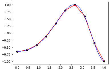
interp2d函数用法与interp1d一样,适用于二维数组。
5. scipy.io文件输入和输出
-
加载和保存
.mat文件- loadmat:加载matlab文件
- savemat:保存为一个matlab文件
- whosmat:列出matlab文件中的变量
示例:
#导入包
import scipy.io as sio
import numpy as np
#保存matlab文件
vect = np.arange(10)
sio.savemat('array.mat',{'vect':vect})
#加载array.mat文件
mat_file = sio.loadmat('array.mat')
print(mat_file)
##输出结果
{'__header__': b'MATLAB 5.0 MAT-file Platform: nt, Created on: Wed Mar 15 19:40:09 2023', '__version__': '1.0', '__globals__': [], 'vect': array([[0, 1, 2, 3, 4, 5, 6, 7, 8, 9]])}

#whosmat的使用
mat_file_content = sio.whosmat('array.mat')
print(mat_file_content)
##输出结果
[('vect', (1, 10), 'int32')]
6. scipy.linalg线性代数
-
导入包
import numpy as np from scipy import linalg -
通过solve函数求解线性方程组ax=b
a = np.array([[3,2,0],[1,-1,0],[0,5,1]]) b = np.array([2,4,-1]) x = linalg.solve(a,b) print(x) ##输出结果 [ 2. -2. 9.] -
通过det函数求行列式
A = np.array([[1,2],[3,4]]) x = linalg.det(A) print(x) ##输出结果 -2.0 -
通过eig函数求方阵的特征根和特征向量
A = np.array([[1,2],[3,4]]) l,v = linalg.eig(A) #l是特征根,v是特征向量 print(l) ##输出结果 [-0.37228132+0.j 5.37228132+0.j] print(v) ##输出结果 [[-0.82456484 -0.41597356] [ 0.56576746 -0.90937671]] -
通过inv函数求方阵的逆
-
通过svd函数对矩阵进行奇异值分解
A = np.random.randn(3,2)
U,S,V = linalg.svd(A)
print(U,S,V)
##输出结果
[[-0.14498216  0.42284152  0.89453073]
 [ 0.20820278 -0.87080259  0.44537003]
 [ 0.96728061  0.25081449  0.03821406]]
[1.81667608 0.36485477]
[[ 0.90137826 -0.43303259]
 [ 0.43303259  0.90137826]]
7. scipy.ndimage图像处理
-
使用misc包里面的图像
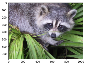
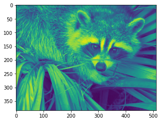
from scipy import misc
f = misc.face()  #使用misc包中的图像
import matplotlib.pyplot as plt
plt.imshow(f)
plt.show()
-
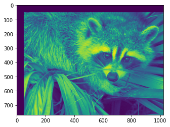
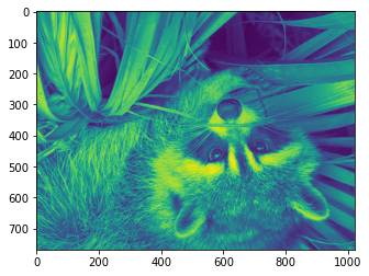
对图像进行几何变换(灰图处理,彩图是三维)
#图像裁剪
face = misc.face(gray = True)
x,y = face.shape
crop_face = face[int(x/4):-int(x/4),int(y/4):-int(y/4)]
plt.imshow(crop_face)
plt.show()

#图片移动
from scipy import ndimage
shift_face = ndimage.shift(face,(50,50),mode = 'constant')
plt.imshow(shift_face)
plt.show()
##mode = {'reflect','constant','nearest','mirror','wrap'}
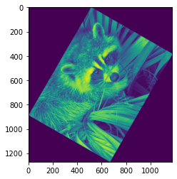
#图片旋转
rotate_face = ndimage.rotate(face,60)
plt.imshow(rotate_face)
plt.show()
#图片缩放
zoom_face = ndimage.zoom(face,0.5)
plt.imshow(zoom_face)
plt.show()
#图片翻转
import numpy as np
flipud_face = np.flipud(face)
plt.imshow(flipud_face)
plt.show()
-
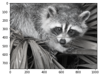
图像过滤
#图像模糊
blurred_face = ndimage.gaussian_filter(f,sigma = 2)
plt.imshow(blurred_face)
plt.show()
##不同的过滤器median_filter
-
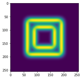
边缘检测
边缘检测用于查找图像内物体的边界,
ndimage提供了一个叫Sobel的函数来进行边缘检测。#示例 im = np.zeros((256, 256)) im[64:-64, 64:-64] = 1 im[90:-90,90:-90] = 2 im = ndimage.gaussian_filter(im, 8) sx = ndimage.sobel(im, axis = 0, mode = 'constant') sy = ndimage.sobel(im, axis = 1, mode = 'constant') sob = np.hypot(sx, sy) plt.imshow(sob) plt.show()
8. scipy.optimize拟合优化
-
拟合
#生成带有噪声的正弦波数据 import numpy as np from scipy import optimize x = np.linspace(-5,5,50) y = 2.9*np.sin(1.5*x) + np.random.randn(50) #定义拟合函数 def test_func(x,a,b): return a*np.sin(b*x) #使用curve_fit拟合曲线 params,params_covariance = optimize.curve_fit(test_func,x,y,p0 = [2,2]) print(params) #输出结果 [3.08974385 1.52187063] -
优化
#求最小值
#定义函数
def f(x):
    return x**2+10*np.sin(x)
x = np.arange(-10,10,0.1)
result = optimize.minimize(f,x0 = 0,method = 'L-BFGS-B')#求函数f的最小值,x0给定起点
print(result)
#输出结果
      fun: array([-7.94582338])
 hess_inv: <1x1 LbfgsInvHessProduct with dtype=float64>
      jac: array([-1.68753901e-06])
  message: 'CONVERGENCE: NORM_OF_PROJECTED_GRADIENT_<=_PGTOL'
     nfev: 12
      nit: 5
     njev: 6
   status: 0
  success: True
        x: array([-1.30644017])
#result中x即为函数最小值
#通过basinhopping函数寻找全局最优解 res = optimize.basinhopping(f,x0 = 0) print(res) -
求标量函数的根
#定义函数
def f(x):
    return x**2+10*np.sin(x)
#求上述方程的根
sol = optimize.root(f,x0 = 0)
print(sol)
#输出结果
   fjac: array([[-1.]])
     fun: array([0.])
 message: 'The solution converged.'
    nfev: 3
     qtf: array([0.])
       r: array([-10.00000001])
  status: 1
 success: True
       x: array([0.])
9. scipy.stats统计函数
-
分布
-
连续型随机变量的概率密度函数(PDF)、累积分布函数(CDF)
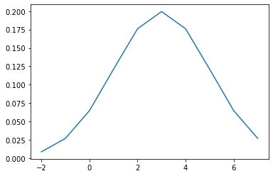
#正态分布
from scipy.stats import norm
#计算多个点的CDF
cdfarr = norm.cdf(np.array([1,-1,0,3,4,6]))
print(cdfarr)
#输出结果
[0.84134475 0.15865525 0.5        0.9986501  0.99996833 1.      ]

#通过百分点函数(PPF,CDF的倒数)找到分位数
ppfvar = norm.ppf(0.25)  #查找标准正态分布的下四分位数
print(ppfvar)
#输出结果
-0.6744897501960817

#计算PDF
bins = np.arange(-2,8)
mean = 3
std = 2
pdf1 = norm.pdf(bins,mean,std)
plt.plot(bins,pdf1)
plt.show()
#若不指定均值和标准差,默认是标准正态分布
-
~~~python
#通过stats.norm.fit拟合出正态分布
samples = np.random.randn(500)
loc,std = norm.fit(samples)
print(loc,std)
#输出结果
0.06709339807973558 1.0022054082150387
~~~

~~~python
#均匀分布
from scipy.stats import uniform
cvar = uniform.cdf([0,1,2,3,4,5],loc = 1,scale = 4)
print(cvar)
#输出结果
[0.   0.   0.25 0.5  0.75 1.  ]
##若不指定loc和scale,默认是0到1上的均匀分布
~~~
-
离散型随机变量的分布律
#二项分布 from scipy.stats import binom cdfv = binom.cdf([0,1,2,3,4,5],n = 3,p = 0.2) print(cdfv) #输出结果 [0.512 0.896 0.992 1. 1. 1. ] -
描述性统计
scipy.stats中的基本统计函数:
函数 描述 describe() 计算描述性统计信息 gmean() 计算沿指定轴的几何平均值 hmean() 计算沿指定轴的谐波平均值 kurtosis() 计算峰度 mode() 返回模态值 skew() 测试数据的偏斜度 f_oneway() 执行单向方差分析 iqr() 计算沿指定轴的数据的四分位数范围 zscore() 计算样本中每个值相对于样本均值和标准偏差的 z值sem() 计算输入数组中值的标准误差(或测量标准误差) -
假设检验
-
单样本均值检验
from scipy import stats #生成服从正态分布的随机变量 rvs = stats.norm.rvs(loc = 5,scale = 6,size = (100,3)) #检验均值是否等于5 sta = stats.ttest_1samp(rvs,5.0) print(sta) #输出结果 Ttest_1sampResult(statistic=array([ 1.34481245, -0.23383869, 0.70731041]), pvalue=array([0.18175869, 0.81559309, 0.48103529])) -
检验两组数据均值是否相等
from scipy import stats
#生成服从正态分布的随机变量
rvs1 = stats.norm.rvs(loc = 5,scale = 6,size = 100)
rvs2 = stats.norm.rvs(loc = 5,scale = 6,size = 100)
#检验两组数据均值是否相等
sta = stats.ttest_ind(rvs1,rvs2)
print(sta)
#输出结果
Ttest_indResult(statistic=-1.6401795251479818, pvalue=0.10255554267049923)
-
10. scipy.special特殊函数
-
立方根函数
from scipy.special import cbrt res = cbrt([10, 9, 3.2, 152]) print (res) #输出结果 [2.15443469 2.08008382 1.4736126 5.3368033 ] -
指数函数
from scipy.special import exp10 #计算10的x次方 res = exp10([2, 4]) print (res) #输出结果 [ 100. 10000.] -
伽马函数
\(x*gamma(x)=gamma(x+1)\)
\(gamma(n+1)=n!\)
from scipy.special import gamma
res = gamma(4)
print(res)
#输出结果
6.0