线性模型
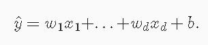
当我们的输入包含d个特征时,我们将预测结果表示为:
向量化:
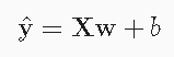
矩阵化:
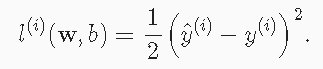
损失函数
平方误差损失函数:
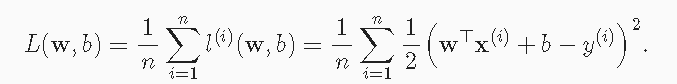
在n个样本上度量:
最优化:
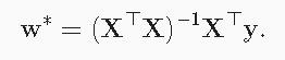
解析解:
随机梯度下降:


矢量化加速
import math
import time
import numpy as np
import tensorflow as tf
import matplotlib.pyplot as plt
from matplotlib_inline import backend_inline
import random
from IPython import display
n = 10000
a = tf.ones([n])
b = tf.ones([n])
# 计时器
class Timer:
    def __init__(self):
        self.times = []
        self.start()

    def start(self):
        self.tik = time.time()

    def stop(self):
        self.times.append(time.time() - self.tik)
        return self.times[-1]

    def avg(self):
        return sum(self.times) / len(self.times)

    def sum(self):
        return sum(self.times)

    def cumsum(self):
        return np.array(self.times).cumsum().tolist()
c = tf.Variable(tf.zeros(n))
timer = Timer()
for i in range(n):
    c[i].assign(a[i] + b[i])
f'{timer.stop():.5f} sec'

"""
'2.87643 sec'
"""

timer.start()
d = a + b
f'{timer.stop():.5f} sec'

"""
'0.00000 sec'
"""
正态分布与平方损失
正态分布概率密度函数:
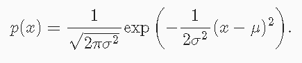
def normal(x, mu, sigma):
p = 1 / math.sqrt(2 * math.pi * sigma ** 2)
return p * np.exp(-0.5 / sigma**2 * (x - mu) ** 2)
def use_svg_display():
backend_inline.set_matplotlib_formats('png')
def set_figsize(figsize=(3.5, 2.5)):
use_svg_display()
plt.rcParams['figure.figsize'] = figsize
def set_axes(axes, xlabel, ylabel, xlim, ylim, xscale, yscale, legend):
"""设置matplotlib的轴"""
axes.set_xlabel(xlabel)
axes.set_ylabel(ylabel)
axes.set_xscale(xscale)
axes.set_yscale(yscale)
axes.set_xlim(xlim)
axes.set_ylim(ylim)
if legend:
axes.legend(legend)
axes.grid()
def plot(X, Y=None, xlabel=None, ylabel=None, legend=None, xlim=None,
ylim=None, xscale='linear', yscale='linear',
fmts=('-', 'm--', 'g-.', 'r:'), figsize=(3.5, 2.5), axes=None):
"""绘制数据点"""
if legend is None:
legend = []
set_figsize(figsize)
axes = axes if axes else plt.gca()
# 如果X有一个轴,输出True
def has_one_axis(X):
return (hasattr(X, "ndim") and X.ndim == 1 or isinstance(X, list)
and not hasattr(X[0], "__len__"))
if has_one_axis(X):
X = [X]
if Y is None:
X, Y = [[]] * len(X), X
elif has_one_axis(Y):
Y = [Y]
if len(X) != len(Y):
X = X * len(Y)
axes.cla()
for x, y, fmt in zip(X, Y, fmts):
if len(x):
axes.plot(x, y, fmt)
else:
axes.plot(y, fmt)
set_axes(axes, xlabel, ylabel, xlim, ylim, xscale, yscale, legend)
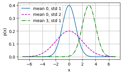
x = np.arange(-7, 7, 0.01)
# 均值和标准差对
params = [(0, 1), (0, 2), (3, 1)]
plot(x, [normal(x, mu, sigma) for mu, sigma in params], xlabel='x', ylabel='p(x)', figsize=(4.5, 2.5),
legend=[f'mean {mu}, std {sigma}' for mu, sigma in params])
plt.show()
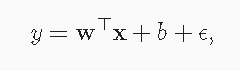
均方误差损失函数可以用于线性回归的一个原因是:我们假设了观测中包含噪声,其中噪声服从正态分布:
根据极大似然估计法:
上述式子的解并不依赖于
σ,因此在高斯噪声的假设下,最小化均方误差等价于对线性模型的极大似然估计。

生成数据集
def synthetic_data(w, b, num_examples):
X = tf.zeros((num_examples, w.shape[0]))
X += tf.random.normal(shape=X.shape)
y = tf.matmul(X, tf.reshape(w, (-1, 1))) + b
y += tf.random.normal(shape=y.shape, stddev=0.01)
y = tf.reshape(y, (-1, 1))
return X, y
true_w = tf.constant([2, -3.4])
true_b = 4.2
features, labels = synthetic_data(true_w, true_b, 1000)
print('features:', features[0], '\nlabel:', labels[0])
"""
features: tf.Tensor([ 0.6943889 -0.36124966], shape=(2,), dtype=float32)
label: tf.Tensor([6.813045], shape=(1,), dtype=float32)
"""
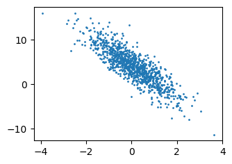
set_figsize()
plt.scatter(features[:, 1].numpy(), labels.numpy(), 1)
读取数据集
def data_iter(batch_size, features, labels):
    num_examples = len(features)
    indices = list(range(num_examples))
    # 这些样本是随机读取的,没有特定的顺序
    random.shuffle(indices)
    for i in range(0, num_examples, batch_size):
        j = tf.constant(indices[i: min(i+batch_size, num_examples)])
        yield tf.gather(features, j), tf.gather(labels, j)

batch_size = 10
for X, y in data_iter(batch_size, features, labels):
    print(X, '\n', y)
    break

"""
tf.Tensor(
[[-0.31621101  0.54274404]
 [-0.5347021   0.2458507 ]
 [ 1.1816338  -1.166924  ]
 [ 0.57692814 -0.8892977 ]
 [-0.4833463  -0.26053128]
 [-0.40469778 -0.53955495]
 [ 0.459481    1.0673087 ]
 [-1.0149183   0.08969461]
 [-0.02690575  0.62452453]
 [ 1.8112805  -1.7324816 ]], shape=(10, 2), dtype=float32)
 tf.Tensor(
[[ 1.7132785]
 [ 2.2795804]
 [10.5091   ]
 [ 8.380901 ]
 [ 4.1135254]
 [ 5.2237015]
 [ 1.4995631]
 [ 1.8668351]
 [ 2.0210123]
 [13.720167 ]], shape=(10, 1), dtype=float32)
"""
初始化模型参数
w = tf.Variable(tf.random.normal(shape=(2, 1), mean=0, stddev=0.01), trainable=True)
b = tf.Variable(tf.zeros(1), trainable=True)
定义模型
def linreg(X, w, b):
    return tf.matmul(X, w) + b
定义损失函数
def squared_loss(y_hat, y):
    return (y_hat - tf.reshape(y, y_hat.shape)) ** 2 / 2
定义优化算法
def sgd(params, grads, lr, batch_size):
    for param, grad in zip(params, grads):
        param.assign_sub(lr * grad / batch_size)
训练
lr = 0.03
num_epochs = 3
net = linreg
loss = squared_loss

for epoch in range(num_epochs):
    for X, y in data_iter(batch_size, features, labels):
        with tf.GradientTape() as g:
            l = loss(net(X, w, b), y)
        # 计算l关于[w, b]的梯度
        dw, db = g.gradient(l, [w, b])
        # 使用参数的梯度更新参数
        sgd([w, b], [dw, db], lr, batch_size)
    train_l = loss(net(features, w, b), labels)
    print(f'epoch {epoch + 1}, loss {float(tf.reduce_mean(train_l)):f}')

"""
epoch 1, loss 0.046574
epoch 2, loss 0.000190
epoch 3, loss 0.000051
"""

print(f'w的估计误差:{true_w - tf.reshape(w, true_w.shape)}')
print(f'b的估计误差:{true_b - b}')

"""
w的估计误差:[-0.00029325 -0.00076914]
b的估计误差:[0.00124931]
"""
线性回归的简单实现
# 生成数据集
true_w = tf.constant([2, -3.4])
true_b = 4.2
features, labels = synthetic_data(true_w, true_b, 1000)

# 读取数据集
def load_array(data_arrays, batch_size, is_train=True):
    dataset = tf.data.Dataset.from_tensor_slices(data_arrays)
    if is_train:
        dataset = dataset.shuffle(buffer_size=1000)
    dataset = dataset.batch(batch_size)
    return dataset

batch_size = 10
data_iter = load_array((features, labels), batch_size)

next(iter(data_iter))

"""
(<tf.Tensor: shape=(10, 2), dtype=float32, numpy=
 array([[ 1.2998679 , -1.8226012 ],
        [ 1.2075672 , -1.4134687 ],
        [-0.2921682 , -0.15664841],
        [-0.8171001 ,  0.50474656],
        [ 0.49231467, -0.51207936],
        [-0.66198266, -0.26582628],
        [-1.556911  , -1.0870522 ],
        [ 0.47099817, -0.18538263],
        [ 1.9214609 ,  0.41514587],
        [-1.4364696 ,  1.447287  ]], dtype=float32)>,
 <tf.Tensor: shape=(10, 1), dtype=float32, numpy=
 array([[13.005127  ],
        [11.413691  ],
        [ 4.137837  ],
        [ 0.84807134],
        [ 6.9113398 ],
        [ 3.7745607 ],
        [ 4.777771  ],
        [ 5.780456  ],
        [ 6.636665  ],
        [-3.5739417 ]], dtype=float32)>)
"""

# 定义模型
net = tf.keras.Sequential()
net.add(tf.keras.layers.Dense(1))

# 初始化模型参数
initializer = tf.initializers.RandomNormal(stddev=0.01)
net = tf.keras.Sequential()
net.add(tf.keras.layers.Dense(1, kernel_initializer=initializer))

# 定义损失函数
loss = tf.keras.losses.MeanSquaredError()

# 定义优化算法
trainer = tf.keras.optimizers.SGD(learning_rate=0.03)

# 训练
num_epochs = 3
net.compile(optimizer=trainer, loss=loss)
net.fit(data_iter, epochs=num_epochs)

"""
Epoch 1/3
100/100 [==============================] - 0s 1ms/step - loss: 1.3062e-04
Epoch 2/3
100/100 [==============================] - 0s 1ms/step - loss: 1.0071e-04
Epoch 3/3
100/100 [==============================] - 0s 1ms/step - loss: 1.0147e-04
<keras.callbacks.History at 0x20be800bfd0>
"""

w = net.get_weights()[0]
print('w的估计误差:', true_w - tf.reshape(w, true_w.shape))
b = net.get_weights()[1]
print('b的估计误差:', true_b - b)

"""
w的估计误差: tf.Tensor([8.7976456e-05 9.8037720e-04], shape=(2,), dtype=float32)
b的估计误差: [0.00094318]
"""
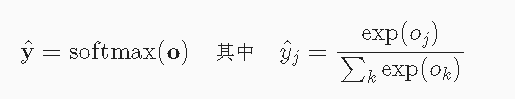
softmax运算
softmax函数能够将未规范化的预测变换为非负数并且总和为1,同时让模型保持可导的性质,softmax运算不会改变未规范化的预测O之间的大小次序,只会确定分配给每个类别的概率。
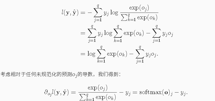
交叉熵损失
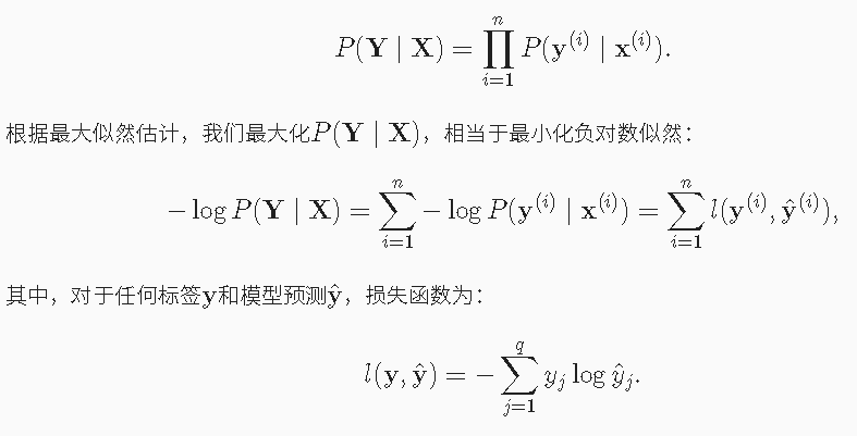
softmax:
softmax回归-图像分类数据集
# 读取数据集
mnist_train, mnist_test = tf.keras.datasets.fashion_mnist.load_data()
len(mnist_train[0]), len(mnist_test[0])
"""
(60000, 10000)
"""
mnist_train[0][0].shape
"""
(28, 28)
"""
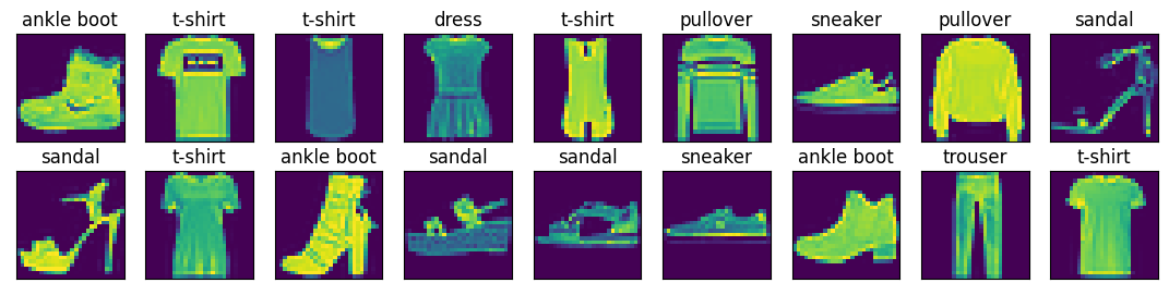
def get_fashion_mnist_labels(labels):
text_labels = ['t-shirt', 'trouser', 'pullover', 'dress', 'coat', 'sandal', 'shirt', 'sneaker', 'bag', 'ankle boot']
return [text_labels[int(i)] for i in labels]
def show_images(imgs, num_rows, num_cols, titles=None, scale=1.5):
figsize = (num_cols * scale, num_rows * scale)
_, axes = plt.subplots(num_rows, num_cols, figsize=figsize)
axes = axes.flatten()
for i, (ax, img) in enumerate(zip(axes, imgs)):
ax.imshow(img.numpy())
ax.axes.get_xaxis().set_visible(False)
ax.axes.get_yaxis().set_visible(False)
if titles:
ax.set_title(titles[i])
plt.show()
return axes
X = tf.constant(mnist_train[0][:18])
y = tf.constant(mnist_train[1][:18])
show_images(X, 2, 9, titles=get_fashion_mnist_labels(y))
# 读取小批量
batch_size = 256
train_iter = tf.data.Dataset.from_tensor_slices(mnist_train).batch(batch_size).shuffle(len(mnist_train[0]))
timer = Timer()
for X, y in train_iter:
continue
f'{timer.stop():.2f} sec'
"""
'0.06 sec'
"""
# 整合所有组件
def load_data_fashion_mnist(batch_size, resize=None):
mnist_train, mnist_test = tf.keras.datasets.fashion_mnist.load_data()
# 将所有数字除以255, 使所有像素值介于0-1之间,在最后添加一个批处理维度
# 并将所有标签转换为int32
process = lambda X, y: (tf.expand_dims(X, axis=3) / 255, tf.cast(y, dtype='int32'))
resize_fn = lambda X, y: (tf.image.resize_with_pad(X, resize, resize) if resize else X, y)
return (
tf.data.Dataset.from_tensor_slices(process(*mnist_train)).batch(batch_size).shuffle(len(mnist_train[0])).map(resize_fn),
tf.data.Dataset.from_tensor_slices(process(*mnist_test)).batch(batch_size).map(resize_fn)
)
train_iter, test_iter = load_data_fashion_mnist(32, resize=64)
for X, y in train_iter:
print(X.shape, X.dtype, y.shape, y.dtype)
break
"""
(32, 64, 64, 1) <dtype: 'float32'> (32,) <dtype: 'int32'>
"""
# 初始化模型参数
num_inputs = 784
num_outputs = 10
W = tf.Variable(tf.random.normal(shape=(num_inputs, num_outputs), mean=0, stddev=0.01))
b = tf.Variable(tf.zeros(num_outputs))
# 定义softmax操作
X = tf.constant([[1.0, 2.0, 3.0], [4.0, 5.0, 6.0]])
tf.reduce_sum(X, 0, keepdims=True), tf.reduce_sum(X, 1, keepdims=True)
"""
(<tf.Tensor: shape=(1, 3), dtype=float32, numpy=array([[5., 7., 9.]], dtype=float32)>,
<tf.Tensor: shape=(2, 1), dtype=float32, numpy=
array([[ 6.],
[15.]], dtype=float32)>)
"""
def softmax(X):
X_exp = tf.exp(X)
partition = tf.reduce_sum(X_exp, 1, keepdims=True)
return X_exp / partition
X = tf.random.normal((2, 5), 0, 1)
X_prob = softmax(X)
X_prob, tf.reduce_sum(X_prob, 1)
"""
(<tf.Tensor: shape=(2, 5), dtype=float32, numpy=
array([[0.17010075, 0.26666152, 0.23135945, 0.06085074, 0.27102757],
[0.06654868, 0.05887584, 0.03383256, 0.41056633, 0.4301766 ]],
dtype=float32)>,
<tf.Tensor: shape=(2,), dtype=float32, numpy=array([1., 1.], dtype=float32)>)
"""
# 定义模型
def net(X):
return softmax(tf.matmul(tf.reshape(X, (-1, W.shape[0])), W) + b)
# 定义损失函数
y_hat = tf.constant([[0.1, 0.3, 0.6], [0.3, 0.2, 0.5]])
y = tf.constant([0, 2])
tf.boolean_mask(y_hat, tf.one_hot(y, depth=y_hat.shape[-1]))
"""
<tf.Tensor: shape=(2,), dtype=float32, numpy=array([0.1, 0.5], dtype=float32)>
"""
def cross_entropy(y_hat, y):
return -tf.math.log(tf.boolean_mask(y_hat, tf.one_hot(y, depth=y_hat.shape[-1])))
cross_entropy(y_hat, y)
"""
<tf.Tensor: shape=(2,), dtype=float32, numpy=array([2.3025851, 0.6931472], dtype=float32)>
"""
# 分类精度
def accuracy(y_hat, y):
if len(y_hat.shape) > 1 and y_hat.shape[1] > 1:
y_hat = tf.argmax(y_hat, axis=1)
cmp = tf.cast(y_hat, y.dtype) == y
return float(tf.reduce_sum(tf.cast(cmp, y.dtype)))
accuracy(y_hat, y) / len(y)
"""
0.5
"""
class Accumulator:
def __init__(self, n):
self.data = [0.0] * n
def add(self, *args):
self.data = [a + float(b) for a, b in zip(self.data, args)]
def reset(self):
self.data = [0.0] * len(self.data)
def __getitem__(self, idx):
return self.data[idx]
def evaluate_accuracy(net, data_iter):
metric = Accumulator(2)
for X, y in data_iter:
metric.add(accuracy(net(X), y), tf.size(y))
return metric[0] / metric[1]
train_iter, test_iter = load_data_fashion_mnist(32)
evaluate_accuracy(net, test_iter)
"""
0.1283
"""
# 训练
def train_epoch_ch3(net, train_iter, loss, updater):
metric = Accumulator(3)
for X, y in train_iter:
with tf.GradientTape() as tape:
y_hat = net(X)
if isinstance(loss, tf.keras.losses.Loss):
l = loss(y, y_hat)
else:
l = loss(y_hat, y)
if isinstance(updater, tf.keras.optimizers.Optimizer):
params = net.trainable_variables
grads = tape.gradient(l, params)
updater.apply_gradients(zip(grads, params))
else:
updater(X.shape[0], tape.gradient(l, updater.params))
# keras的loss默认返回一个批量的平均损失
l_sum = l * float(tf.size(y)) if isinstance(loss, tf.keras.losses.Loss) else tf.reduce_sum(l)
metric.add(l_sum, accuracy(y_hat, y), tf.size(y))
return metric[0] / metric[2], metric[1] / metric[2]
class Animator:
def __init__(self, xlabel=None, ylabel=None, legend=None, xlim=None, ylim=None, xscale='linear', yscale='linear',
fmts=('-', 'm--', 'g-.', 'r:'), nrows=1, ncols=1, figsize=(3.5, 2.5)):
# 增量地绘制多条线
if legend is None:
legend = []
use_svg_display()
self.fig, self.axes = plt.subplots(nrows, ncols, figsize=figsize)
if nrows * ncols == 1:
self.axes = [self.axes, ]
# 使用lambda函数捕获参数
self.config_axes = lambda: set_axes(self.axes[0], xlabel, ylabel, xlim, ylim, xscale, yscale, legend)
self.X, self.Y, self.fmts = None, None, fmts
def add(self, x, y):
# 向图中添加多个数据点
if not hasattr(y, "__len__"):
y = [y]
n = len(y)
if not hasattr(x, "__len__"):
x = [x] * n
if not self.X:
self.X = [[] for _ in range(n)]
if not self.Y:
self.Y = [[] for _ in range(n)]
for i, (a, b) in enumerate(zip(x, y)):
if a is not None and b is not None:
self.X[i].append(a)
self.Y[i].append(b)
self.axes[0].cla()
for x, y, fmt in zip(self.X, self.Y, self.fmts):
self.axes[0].plot(x, y, fmt)
self.config_axes()
display.display(self.fig)
display.clear_output(wait=True)
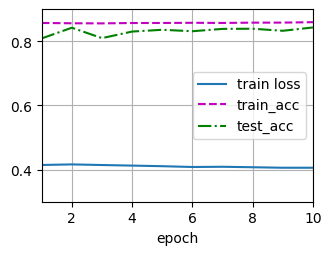
def train_ch3(net, train_iter, test_iter, loss, num_epochs, updater):
animator = Animator(xlabel='epoch', xlim=[1, num_epochs], ylim=[0.3, 0.9], legend=['train loss', 'train_acc', 'test_acc'])
for epoch in range(num_epochs):
train_metrics = train_epoch_ch3(net, train_iter, loss, updater)
test_acc = evaluate_accuracy(net, test_iter)
animator.add(epoch+1, train_metrics + (test_acc,))
train_loss, train_acc = train_metrics
assert train_loss < 0.5, train_loss
assert train_acc <= 1 and train_acc > 0.7, train_acc
assert test_acc <=1 and test_acc > 0.7, test_acc
class Updater:
def __init__(self, params, lr):
self.params = params
self.lr = lr
def __call__(self, batch_size, grads):
sgd(self.params, grads, self.lr, batch_size)
updater = Updater([W, b], lr=0.1)
num_epochs = 10
train_ch3(net, train_iter, test_iter, cross_entropy, num_epochs, updater)
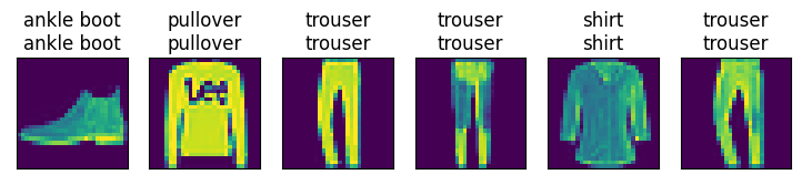
# 预测
def predict_ch3(net, test_iter, n=6):
    for X, y in test_iter:
        break
    trues = get_fashion_mnist_labels(y)
    preds = get_fashion_mnist_labels(tf.argmax(net(X), axis=1))
    titles = [true + '\n' + pred for true, pred in zip(trues, preds)]
    show_images(tf.reshape(X[0:n], (n, 28, 28)), 1, n, titles=titles[0:n])

predict_ch3(net, test_iter)
# Keras高层API
# 初始化模型参数
batch_size = 256
train_iter, test_iter = load_data_fashion_mnist(batch_size)

net = tf.keras.models.Sequential()
net.add(tf.keras.layers.Flatten(input_shape=[28, 28]))
weight_initializer = tf.keras.initializers.RandomNormal(mean=0.0, stddev=0.01)
net.add(tf.keras.layers.Dense(10, kernel_initializer=weight_initializer))

# 重新审视softmax的实现
loss = tf.keras.losses.SparseCategoricalCrossentropy(from_logits=True)

# 优化算法
trainer = tf.keras.optimizers.SGD(learning_rate=.1)

# 训练
num_epochs = 10
train_ch3(net, train_iter, test_iter, loss, num_epochs, trainer)
