技术背景

所谓的近邻表求解，就是给定N个原子的体系，找出满足cutoff要求的每一对原子。在前面的几篇博客中，我们分别介绍过CUDA近邻表计算与JAX-MD关于格点法求解近邻表的实现。虽然我们从理论上可以知道，用格点法求解近邻表，在复杂度上肯定是要优于传统的算法。本文主要从Python代码的实现上来具体测试一下二者的速度差异，这里使用的硬件还是CPU。

算法解析

若一对原子A和B满足下述条件，则称A、B为一对近邻原子：

\[|\textbf{r}_A-\textbf{r}_B|\leq cutoff \]

传统的求解方法，就是把所有原子间距都计算一遍，然后对每个原子的近邻原子进行排序，最终按照给定的cutoff截断值确定相关的近邻原子。在Python中的实现，因为有numpy这样的强力工具，我们在计算原子两两间距时，只需要对一组维度为(N,D)的原子坐标进行扩维，分别变成(1,N,D)和(N,1,D)大小的原子坐标。然后将二者相减，计算过程中会自动广播(Broadcast)成(N,N,D)和(N,N,D)的两个数组进行计算。对得到的结果做一个Norm，就可以得到维度为(N,N)的两两间距矩阵。该算法的计算复杂度为O(N^2)。

相对高效的一种求解方案是将原子坐标所在的空间划分成众多的小区域，通常我们设定这些小区域为边长等于cutoff的小正方体。这种设定有一个好处是，我们可以确定每一个正方体的近邻原子，一定在最靠近其周边的26个小正方体区域内。这样一来，我们就不需要去计算全局的两两间距，只需要计算单个小正方体内(假定有M个原子)的两两间距(M,M)，以及单个正方体与周边正方体内原子的配对间距(M,26M)。之所以这样分开计算，是为了减少原子跟自身间距的这一项重复计算。那么对于整个空间的原子，就需要计算(N,27M)这么多次的原子间距，是一个复杂度为O(NlogN)的算法。

Numpy代码实现

这里我们基于Python中的numpy框架来实现这两个不同的计算近邻表的算法。其实当我们使用numpy来进行计算的时候，应当尽可能的避免循环体的使用。但是这里仅演示两种算法的差异性，因此在实现格点法的时候偷了点懒，用了两个for循环，感兴趣的童鞋可以自行优化。

import time
from itertools import chain
from operator import itemgetter
import numpy as np

# 在格点法中，为了避免重复计算，我们可以仅计算一半的近邻格点中的原子间距
NEIGHBOUR_GRID = np.array([
       [-1,  1,  0],
       [-1, -1,  1],
       [-1,  0,  1],
       [-1,  1,  1],
       [ 0, -1,  1],
       [ 0,  0,  1],
       [ 0,  1,  0],
       [ 0,  1,  1],
       [ 1, -1,  1],
       [ 1,  0,  0],
       [ 1,  0,  1],
       [ 1,  1,  0],
       [ 1,  1,  1]], np.int32)

# 原始的两两间距计算方法，需要排序
def get_neighbours_by_dist(crd, cutoff):
    large_dis = np.tril(np.ones((crd.shape[0], crd.shape[0])) * 999)
    # (N, N)
    dis = np.linalg.norm(crd[None] - crd[:, None], axis=-1) + large_dis
    # (N, M)
    neigh = np.argsort(dis, axis=-1)
    # (N, M)
    cut = np.take_along_axis(dis, neigh, axis=1)
    # (2, P)
    pairs = np.where(cut <= cutoff)
    # (P, )
    pairs_id0 = pairs[0]
    pairs_id1 = neigh[pairs]
    # (P, 2)
    sort_args = np.argsort(pairs_id0)
    return np.hstack((pairs_id0[..., None], pairs_id1[..., None]))[sort_args]

# 格点法计算近邻表，先分格点，然后分两个模块计算单格点内原子间距，和中心格点-周边格点内的原子间距
def get_neighbours_by_grid(crd, cutoff):
    # (D, )
    min_xyz = np.min(crd, axis=0)
    max_xyz = np.max(crd, axis=0)
    space = max_xyz - min_xyz
    grids = np.ceil(space / cutoff).astype(np.int32)
    num_grids = np.product(grids)
    buffer = (grids * cutoff - space) / 2
    start_crd = min_xyz - buffer
    # (N, D)
    grid_id = ((crd - start_crd) // cutoff).astype(np.int32)
    grid_coe = np.array([1, grids[0], grids[1]], np.int32)
    # (N, )
    grid_id_1d = np.sum(grid_id * grid_coe, axis=-1).astype(np.int32)
    # (N, 2)
    grid_id_dict = np.ndenumerate(grid_id_1d)
    # (G, *)
    grid_dict = dict.fromkeys(range(num_grids), ())
    for index, value in grid_id_dict:
        grid_dict[value] += index
    neighbour_grid = (NEIGHBOUR_GRID * grid_coe).sum(axis=-1).astype(np.int32)
    neighbour_pairs = []

    for i in range(num_grids):
        if grid_dict[i]:
            keeps = np.where((neighbour_grid + i < num_grids) & (neighbour_grid + i >= 0))[0]
            neighbour_grid_keep = neighbour_grid[keeps] + i
            grid_atoms = np.array(list(grid_dict[i]), np.int32)
            try:
                grid_neighbours = np.array(list(chain(*itemgetter(*neighbour_grid_keep)(grid_dict))), np.int32)
            except TypeError:
                if neighbour_grid_keep.size == 0:
                    grid_neighbours = np.array([], np.int32)
                else:
                    grid_neighbours = np.array(list(itemgetter(*neighbour_grid_keep)(grid_dict)), np.int32)
            grid_crds = crd[grid_atoms]
            grid_neighbour_crds = crd[grid_neighbours]
            large_dis = np.tril(np.ones((grid_crds.shape[0], grid_crds.shape[0])) * 999)
            # 单格点内部原子间距
            grid_dis = np.linalg.norm(grid_crds[None] - grid_crds[:, None], axis=-1) + large_dis
            grid_pairs = np.argsort(grid_dis, axis=-1)
            grid_cut = np.take_along_axis(grid_dis, grid_pairs, axis=-1)
            pairs = np.where(grid_cut <= cutoff)
            pairs_id0 = grid_atoms[pairs[0]]
            pairs_id1 = grid_atoms[grid_pairs[pairs]]
            neighbour_pairs.extend(list(np.hstack((pairs_id0[..., None], pairs_id1[..., None]))))
            # 中心格点-周边格点内原子间距
            grid_dis = np.linalg.norm(grid_crds[:, None] - grid_neighbour_crds[None], axis=-1)
            grid_pairs = np.argsort(grid_dis, axis=-1)
            grid_cut = np.take_along_axis(grid_dis, grid_pairs, axis=-1)
            pairs = np.where(grid_cut <= cutoff)
            pairs_id0 = grid_atoms[pairs[0]]
            pairs_id1 = grid_neighbours[grid_pairs[pairs]]
            neighbour_pairs.extend(list(np.hstack((pairs_id0[..., None], pairs_id1[..., None]))))
    neighbour_pairs = np.sort(np.array(neighbour_pairs), axis=-1)
    sort_args = np.argsort(neighbour_pairs[:, 0])
    return neighbour_pairs[sort_args]

# 时间测算函数
def benchmark(N, cutoff=0.3, D=3):
    crd = np.random.random((N, D)).astype(np.float32) * np.array([3., 4., 5.], np.float32)
    # Solution 1
    time0 = time.time()
    neighbours_1 = get_neighbours_by_dist(crd, cutoff)
    time1 = time.time()
    record_1 = time1 - time0
    # Solution 2
    time0 = time.time()
    neighbours_2 = get_neighbours_by_grid(crd, cutoff)
    time1 = time.time()
    record_2 = time1 - time0
    for pair in neighbours_1:
        if (np.isin(neighbours_2, pair).sum(axis=-1) < 2).all():
            print (pair)
    assert neighbours_1.shape == neighbours_2.shape
    return record_1, record_2

# 绘图主函数
if __name__ == '__main__':
    import matplotlib.pyplot as plt
    sizes = range(1000, 10000, 1000)
    time_dis = []
    time_grid = []
    for size in sizes:
        print (size)
        times = benchmark(size)
        time_dis.append(times[0])
        time_grid.append(times[1])

    plt.figure()
    plt.title('Neighbour List Calculation Time')
    plt.plot(sizes, time_dis, color='black', label='Full Connect')
    plt.plot(sizes, time_grid, color='blue', label='Cell List')
    plt.xlabel('Size')
    plt.ylabel('Time/s')
    plt.legend()
    plt.grid()
    plt.show()

上述代码的运行结果如下图所示：

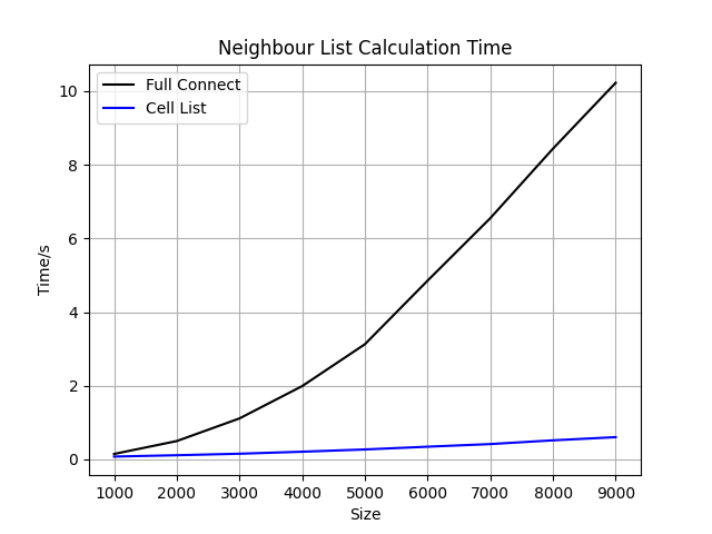
其实因为格点法中使用了for循环的问题，函数效率并不高。因此在体系非常小的场景下(比如只有几十个原子的体系)，本文用到的格点法代码效率并不如计算所有的原子两两间距。但是毕竟格点法的复杂度较低，因此在运行过程中随着体系的增长，格点法的优势也越来越大。

近邻表计算与分子动力学模拟

在分子动力学模拟中计算长程相互作用时，会经常使用到近邻表。如果要在GPU上实现格点近邻算法，有可能会遇到这样的一些问题：

GPU更加擅长处理静态Shape的张量，因此往往会使用一个最大近邻数，对每一个原子的近邻原子标号进行限制，一般不允许满足cutoff的近邻原子数超过最大近邻数，否则这个cutoff就失去意义了。而如果单个原子的近邻原子数量低于最大近邻数，这时候就会用一个没有意义的数对剩下分配好的张量空间进行填充(Padding)，这样一来会带来很多不必要的计算。
在运行分子动力学模拟的过程中，体系原子的坐标在不断的变化，近邻表也会随之变化，而此时的最大近邻数有可能无法存储完整的cutoff内的原子。

总结概要

本文介绍了在Python的numpy框架下计算近邻表的两种不同算法的原理以及复杂度，另有分别对应的两种代码实现。在实际使用中，我们更偏向于第二种算法的使用。因为对于第一种算法来说，哪怕是一个10000个原子的小体系，如果要计算两两间距，也会变成10000*10000这么大的一个张量的运算。可想而知，这样计算的效率肯定是比较低下的。