pytorch损失函数
| 损失函数 | 名称 | 场景 |
|---|---|---|
| nn.MSELoss() | 均方误差损失(MSE) | 回归 |
| nn.L1Loss() | 平均绝对误差损失(MAE) | 回归 |
| nn.SmoothL1Loss() | 平滑L1损失 | 回归 |
| nn.HuberLoss() | Huber损失,平滑平均绝对误差 | 回归 |
| nn.BCELoss() | 二分类交叉熵,结合sigmoid函数使用 | 分类 |
| nn.BCEWithLogitsLoss() | 二分分类交叉熵 | 分类 |
| nn.CrossEntropyLoss() | 多分类交叉熵损失函数 | 分类 |
| nn.NLLLoss() | 负对数似然损失,结合结合log softmax使用 | 分类 |
| nn.CosineSimilarity() | 余弦相似度 | 计算距离 |
均方误差            L2 范数  nn.MSELoss()
平均绝对误差         L1 范数  nn.L1Loss()

Smooth L1 Loss     Smooth L1 Loss   nn.SmoothL1Loss()
Huber损失           HuberLoss        nn.HuberLoss()

KL散度损失                           nn.KLDivLoss()
负对数似然损失                        nn.NLLLoss()

二分类交叉熵损失     nn.BCELoss()
多类别交叉熵损失     nn.CrossEntropyLoss()

余弦相似度损失
损失函数概念
损失函数: 衡量模型输出与真实标签的差异。
通常,说到损失函数会出现3个概念
(1)损失函数(Loss Function):计算单样本的差异
(2)代价函数(Cost Function):计算整个训练集、样本集(所有样本)Loss的平均值、
(3)目标函数(Objective Function):训练模型的最终目标—目标包含cost和Regularization
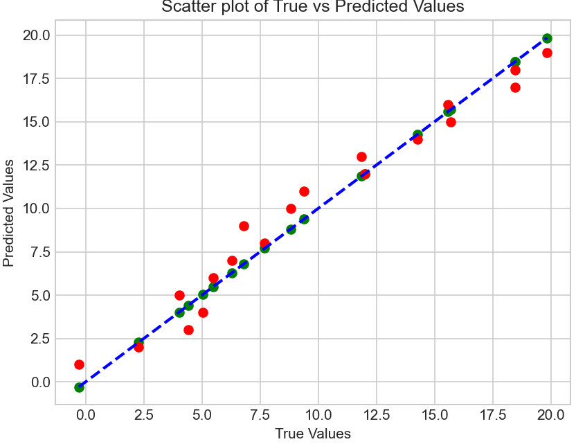
均方误差损失Mean Squared Error,MSE
均方误差是一种常用的损失函数,通常用于衡量回归模型预测结果与真实值之间的差异程度。
均方误差是通过计算预测值与真实值之间差异的平方和来衡量模型的性能。
它对于较大的差异给予更高的权重,因为平方操作会放大较大的差异。
均方误差的数值越小,表示模型预测的结果与真实值越接近。
公式如下
# torch 损失函数
torch.nn.MSELoss(*size_average=None*, *reduce=None*, *reduction='mean'*)
import numpy as np
import matplotlib.pyplot as plt
import torch
import torch.nn as nn

plt.style.use("seaborn-v0_8-whitegrid")

# 真实值和预测值  y_true,y_pred
y_pred = np.array(range(1,20))
y_true = y_pred + np.random.randn(19)

# 计算均方误差
mse = np.mean((y_true - y_pred) ** 2)
print("MSE:", mse)

# torch
mseloss=nn.MSELoss()
mse=mseloss.forward(torch.tensor(y_true),torch.tensor(y_pred))
print("mse",mse)

# 绘制真实值和预测值的散点图
plt.scatter(y_true, y_true,c="g")
plt.scatter(y_true, y_pred,c="r")

plt.plot([min(y_true), max(y_true)], [min(y_true), max(y_true)], 'k--',c="b", lw=2)  # 绘制直线y=x
plt.xlabel('True Values')
plt.ylabel('Predicted Values')
plt.title('Scatter plot of True vs Predicted Values')
plt.show()

# MSE: 1.3939309147057835
# mse tensor(1.3939, dtype=torch.float64)
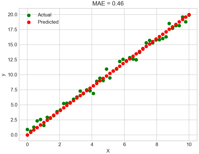
平均绝对误差损失Mean Absolute Error, MAE
平均绝对误差(Mean Absolute Error,MAE)是一种用于衡量预测模型性能的损失函数,通常用于回归问题。
它衡量了模型的预测值与实际观测值之间的平均绝对差异。MAE 的值越小,表示模型的预测越准确。
MAE 的原理非常简单,它是所有绝对误差的平均值。绝对误差是指每个观测值的预测值与实际值之间的差的绝对值。
MAE 的计算过程非常直观,它将每个样本的绝对误差取绝对值后求平均,因此它对异常值不敏感。
平均绝对误差的计算公式:
# torch 损失函数
criterion = nn.L1Loss()
import numpy as np
import matplotlib.pyplot as plt
import torch
import torch.nn as nn

plt.style.use("seaborn-v0_8-whitegrid")

# 生成随机数据
np.random.seed(0)
n = 50
X = np.linspace(0, 10, n)
# y_true y_pred
y_pred = 2 * X   # 模拟的预测值
y_true = 2 * X  + np.random.normal(0, 1, n) * 0.5   # 真实的目标值,包含随机噪音
# 计算MAE
mae = np.mean(np.abs(y_true - y_pred))

# torch 计算
maeloss= nn.L1Loss()
maetorch=maeloss(torch.tensor(y_true),torch.tensor(y_pred))
print(mae,maetorch)

# 绘制数据点和预测线
plt.scatter(X, y_true, label='Actual', color='g')
plt.scatter(X, y_pred, label='Predicted', color='r')
plt.title(f'MAE = {mae:.2f}')
plt.xlabel('X')
plt.ylabel('y')
plt.legend()
plt.show()

# 0.45699838217894007 tensor(0.4570, dtype=torch.float64)
平滑L1损失,Smooth L1 Loss
Smooth L1 结合了 MSE 和 MAE 的优点,来自 Fast R-CNN 论文
当真实值和预测值之间的绝对差低于 β  时,使用 MSE 损失。
MSE 损失曲线是一条连续曲线,这意味着每个损失值处的梯度都会变化,并且可以在任何地方可导。
然而,对于非常大的损失值,梯度爆炸,使用平均绝对误差,
当绝对差变得大于 β 并且消除了潜在的梯度爆炸时,其梯度对于每个损失值几乎是恒定的。
torch.nn.SmoothL1Loss(size_average=None, *reduce=None, reduction='mean', beta=1.0)
import torch

loss = torch.nn.SmoothL1Loss()
input = torch.randn(3, 5, requires_grad=True)
target = torch.randn(3, 5)
output1 = loss(input, target)
print('output1: ',output1)
# output1:  tensor(0.7812, grad_fn=<SmoothL1LossBackward0>)
平滑平均绝对误差,Huber损失
Huber损失又称平滑平均绝对误差
Huber损失是一种用于回归问题的损失函数, 使用 detla 进行了缩放,结合L1Loss和MSELoss的优点
它对异常值不敏感,相比于均方误差(MSE),它对异常值的惩罚较小。
Huber损失的主要思想是在距离真实值较近的情况下采用均方误差,而在距离较远的情况下采用绝对误差,当δ趋向于0时它就退化成了MAE,而当δ趋向于无穷时则退化为了MSE
这种权衡可以有效减少异常值的影响。
torch.nn.HuberLoss(reduction='mean', delta=1.0)
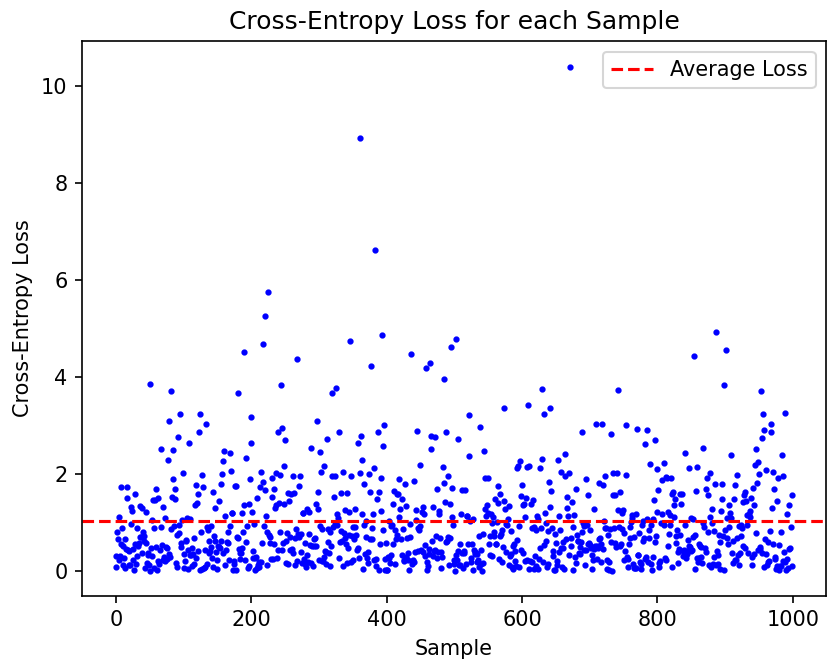
交叉熵损失Cross-Entropy Loss
交叉熵损失(Cross-Entropy Loss)是机器学习中常用的一种损失函数,主要应用于分类问题。
它用于衡量模型预测结果与实际标签之间的差异。
交叉熵损失基于信息论中的交叉熵概念,用于度量两个概率分布之间的相似性。
在分类问题中,我们将实际标签表示为一个one-hot向量,即只有一个元素为1,其余元素为0;而模型的预测结果通常是一个概率分布。
交叉熵损失通过计算实际标签和模型预测结果之间的交叉熵来评估模型的性能。
交叉熵:它主要刻画的是实际输出(概率)与期望输出(概率)的距离,也就是交叉熵的值越小,两个概率分布就越接近
其中 为实际标签中第个类别的概率(one-hot编码),为模型预测的第个类别的概率。
import numpy as np
import matplotlib.pyplot as plt

def cross_entropy_loss(y_true, p_pred):
    epsilon = 1e-10  # 添加一个小的常数以避免log(0)计算错误
    return -np.sum(y_true * np.log(p_pred + epsilon), axis=1)

# 模拟数据
num_samples = 1000
num_classes = 5

np.random.seed(42)
y_true = np.eye(num_classes)[np.random.choice(num_classes, num_samples)]  # 生成随机的one-hot标签
p_pred = np.random.rand(num_samples, num_classes)  # 模型预测的概率

loss = cross_entropy_loss(y_true, p_pred)

# 计算平均损失
average_loss = np.mean(loss)

# 绘制损失函数图形
plt.plot(range(num_samples), loss, 'bo', markersize=2)
plt.xlabel('Sample')
plt.ylabel('Cross-Entropy Loss')
plt.title('Cross-Entropy Loss for each Sample')
plt.axhline(average_loss, color='r', linestyle='--', label='Average Loss')
plt.legend()
plt.show()

print(f'Average Loss: {average_loss}')
二分类交叉熵损失:

criterion = nn.BCELoss()

多类别交叉熵损失:
torch.nn.CrossEntropyLoss(*weight=None*, *size_average=None*, *ignore_index=- 100*, *reduce=None*, *reduction='mean'*, *label_smoothing=0.0*)
KL散度损失Kullback-Leibler Divergence Loss
通常在生成模型中使用,用于测量两个概率分布之间的差异。
criterion = nn.KLDivLoss()
import  numpy as np
import torch
import torch.nn.functional as F
import torch.nn as nn

kl_loss = nn.KLDivLoss(reduction="batchmean")
# input should be a distribution in the log space
input1 = F.log_softmax(torch.randn(3, 5, requires_grad=True), dim=1)
# Sample a batch of distributions. Usually this would come from the dataset
input2 = torch.rand(3, 5)
print(input1)

target = F.softmax(input2, dim=1)
output = kl_loss(input1, target)

print(output)

kl_loss = nn.KLDivLoss(reduction="batchmean", log_target=True)
log_target = F.log_softmax(input2, dim=1)
output = kl_loss(input1, log_target)

print(output)

# tensor([[-3.1245, -0.4438, -2.7561, -2.9293, -1.6223],
#         [-1.6743, -2.2721, -1.2506, -0.9937, -2.9387],
#         [-1.0872, -2.4577, -1.0433, -1.6925, -3.1981]],
#        grad_fn=<LogSoftmaxBackward0>)
# tensor(0.4822, grad_fn=<DivBackward0>)
# tensor(0.4822, grad_fn=<DivBackward0>)
负对数似然损失(Negative Log Likelihood Loss)
Negative Log-Likelihood (NLL) 损失函数的工作原理与交叉熵损失函数非常相似
NLL要求网络最后一层使用 softmax 作为激活函数。通过softmax将输出值映射为每个类别的概率值。
criterion = nn.NLLLoss()
import  numpy as np
import torch
import torch.nn.functional as F
import torch.nn as nn

m = nn.LogSoftmax(dim=1)
loss = nn.NLLLoss()
# input is of size N x C = 3 x 5
input = torch.randn(3, 5, requires_grad=True)
# each element in target has to have 0 <= value < C
target = torch.tensor([1, 0, 4])
output = loss(m(input), target)
print(output)
# tensor(1.6105, grad_fn=<NllLossBackward0>)

# 案例2
# 2D loss example (used, for example, with image inputs)
N, C = 5, 4
loss = nn.NLLLoss()
# input is of size N x C x height x width
data = torch.randn(N, 16, 10, 10)
conv = nn.Conv2d(16, C, (3, 3))
m = nn.LogSoftmax(dim=1)
# each element in target has to have 0 <= value < C
target = torch.empty(N, 8, 8, dtype=torch.long).random_(0, C)
output = loss(m(conv(data)), target)
print(output)
# tensor(1.5389, grad_fn=<NllLoss2DBackward0>)
余弦相似度损失Cosine Similarity Loss
余弦相似度损失是一种常用的机器学习损失函数,用于衡量向量之间的相似性。
它基于向量的内积和范数来计算相似度,并将其转化为一个损失值。
余弦相似度损失基于余弦相似度的概念。余弦相似度是两个向量之间的夹角的余弦值,范围在-1到1之间。
当夹角为0度时,余弦相似度为1,表示两个向量完全相同;
当夹角为90度时,余弦相似度为0,表示两个向量无关;
当夹角为180度时,余弦相似度为-1,表示两个向量完全相反。
# nn.CosineSimilarity(dim=1, eps=1e-08)
import torch
import torch.nn as nn
import torch.nn.functional as F

batch_sz = 5; num_feat = 128
loss_fn = torch.nn.CosineEmbeddingLoss()
v1 = torch.randn(batch_sz, num_feat)
v2 = torch.randn(batch_sz, num_feat)
target = torch.randint(2, size=(batch_sz,))*2 -1
res = loss_fn(v1, v2, target)
print(res)
# # tensor(0.3383)
参考资料
https://pytorch.org/docs/stable/nn.html#loss-functions 官网
https://mp.weixin.qq.com/s/vzh1We1rNVv1ZFWsxYTGMA
https://mp.weixin.qq.com/s/ugFeeHJlRerSwjygaXpOaQ
https://mp.weixin.qq.com/s/U8Bixzp1U4RoEz1W_YKhOQ