结果

代码

clear all;close all;clc;
% Define the range for n and m
n_values = 0:5;
pixels=100;%image x,y pixels

%%The transverse and longitudinal dimensions of the pupil surface
% can enhance the Fourier transform results by reducing the proportion of pupil area
q=300;   



% Initialize a figure
fig=figure('name','ZernikePolynomials');
figWidth = 620; % Set the figure width
figHeight = 620; % Set the figure height
set(fig, 'Position', [200, 200, figWidth, figHeight]);


%% Creating mask for unit circle
X = linspace(-1, 1, pixels);
[X, Y] = meshgrid(X, X);
circleMask = (X.^2 + Y.^2) <= 1;


% Loop over n values
for i = 1:length(n_values)
    n = n_values(i);

    % Loop over m values, incrementing by 2
    for m = -n:2:n
        % Calculate index for the subplot
        subplot_index = (i-1)*(n+1) + (m+n)/2 + 1;

        % Calculate radial polynomial
        [RmnC,rhoExp] = calcRmn(abs(m),n);
        % Calculate zernike polynomial as raster scan
        myData = zeros(pixels);
        myData = calcZP(RmnC,rhoExp,m,n,pixels);

        % Apply mask to myData
        myData(~circleMask) = NaN;

        
        % Create subplot
        margin=0.04; % Adjust this to control the spacing between subplots
        subplot_tight(length(n_values), n+1, subplot_index, margin);
        imagesc(myData);
        axis square;
        colormap("jet");
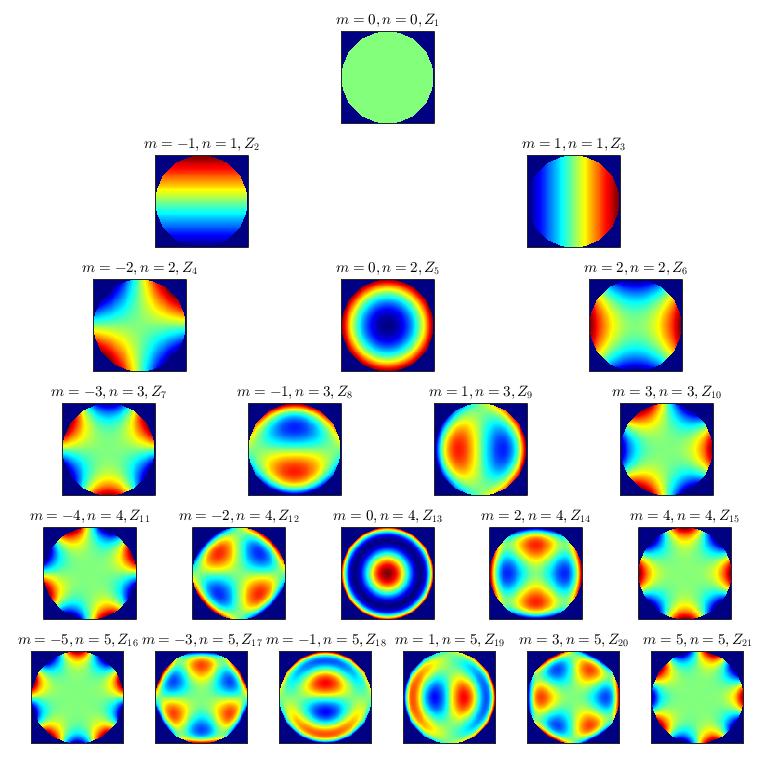
        title(['$m=' num2str(m) ', n=' num2str(n) ', Z_{' num2str(subplot_index-(1+n)*n/2 ) '}$'], 'Interpreter', 'latex');

        % Remove x and y labels
        set(gca,'xtick',[],'ytick',[]);
    end
end


%%
function [PC,PExp]=calcRmn (m,n)
%CALCRMN calculate the radial polynomial
%Inputs Zernike polynomial values m,n
%Returns the coefficients for polynomial exponents
%Parameters
OET=(n-m);%check if odd or even
mC=OET/2;%number of coefficients calculated
%Initialize
RmnC= zeros(1,mC);
rhoExp=zeros(1,mC);
%Calculation of radial polynomial
if mod(OET,2)==0
    %do if test is even;otherwise dont
    k=0;Rmn=0;
    while k<=mC
        Rmn=(-1)^k*factorial(n-k)/(factorial(k)*factorial((n+m)/2-k)*factorial((n-m)/2-k));
        k=k+1;
        PC(k)=Rmn;%Polynomial coefficients
        PExp(k)=(n-2*(k-1));%Polynomial exponents
    end
end
end%End function

function mD =calcZP(RmnC,rhoExp,m,n,pX)
%CALCZP calculate the zernike polynomial shape
%Inputs radial polynomial,plus m,n,pixels
%Returns the Zernike polynomial data set
%Calculate Zernike polynomial shape


mD=zeros(pX);
for r=1:pX
    for c=1:pX
        x=(2*c-pX-1)/pX;%convert to x,y
        y=(2*r-pX-1)/pX;%convert to x,y
        %Calculate quadrant correct angle
        phi=atan2(y,x);
        %Convert rectangular coord to distance
        rho=sqrt(x^2+y^2);
        RMN =0;
        for count =1:(n-abs(m))/2+1
            RMN =RMN+RmnC(count)*rho.^rhoExp(count);
        end
        %Calculate ZP wavefront
        if m<0 || n==0   %select for+/-m
            Z=-RMN*sin(abs(m)*phi);
        else
            Z=RMN*cos(abs(m)*phi);
        end
        %Control visual appearance
        if rho<=1%zero outside unit circle
            mD(r,c)=Z;%load value
        else
            mD(r,c)=0;%change to Nan to hide
        end
    end
end
end%End Function