ECOD: Unsupervised Outlier Detection Using Empirical Cumulative Distribution Functions
Author:Zheng Li, Yue Zhao, Student Member Xiyang Hu, Nicola Botta, Cezar Ionescu, and George H. Chen
Journal:IEEE TRANSACTIONS ON KNOWLEDGE AND DATA ENGINEERING
Contribution
- Propose a novel outlier detection method called ECOD, which is both parameter-free and easy to interpret
- perform extensive experiments on 30 benchmark datasets, where we find that ECOD outperforms 11 state-of-the-art baselines in terms of accuracy, efficiency, and scalability
- release an easy-to-use and scalable (with distributed support) Python implementation for accessibility and reproducibility.
Introduction
These existing approaches have a few limitations:
- The models requiring density estimation and pairwise distance calculation suffer from the curse of dimensionality
- Most methods require hyperparameter tuning, which is difficult in the unsupervised setting
ECOD(Empirical-Cumulative-distribution-based Outlier Detection) is inspired by the fact that outliers are often the “rare events” that appear in the tails of a distribution.
Rare events are often the ones that appear in one of the tails of a distribution.
As a concrete example, if the data are sampled from a one-dimensional Gaussian, then points in the left or right tails are often considered to be the rare events or outliers.
The "three-sigma" rule declares points more than three standard deviations from the mean to be outliers
We compute a univariate ECDF for each dimension separately. Then to measure the outlyingness of a data point, we compute its tail probability across all dimensions via an independence assumption, which amounts to multiplying all the estimated tail probabilities from the different univariate ECDFs
Algorithm
Problem Formulation
We consider the following standard unsupervised outlier detection (UOD) setup.
We assume that we have \(n\) data points \(X_1,X_2,\dots,X_n \in \mathbb{R}^d\) that are sampled i.i.d.(Independent and identically distributed)
We collectively refer to this entire dataset by the matrix \(\boldsymbol{X} \in \mathbb{R}^{n\times d}\) , which is formed by stacking the different data points’ vectors as rows.
Given \(\boldsymbol{X}\), an OD model M assigns, for each data point \(X_i\) , an outlier score \(O_i \in\mathbb{R}\) (higher means more likely an outlier).
joint cumulative distribution function (CDF)
let \(F:\mathbb{R}^d \rightarrow [0,1]\) denote the joint cumulative distribution function (CDF) across all \(d\) dimensions/features.
In particular, \(X_1,X_2,\dots,X_n\) are assumed to be sampled i.i.d. from a distribution with joint CDF F.
For a vector \(z\in\mathbb{R}^d\) , we denote its \(j\)-th entry as \(z^{(j)}\) , e.g., we write the \(j\)-th entry of \(X_i\) as \(X_i^{(j)}\) .
We use the random variable \(X\) to denote a generic random variable with the same distribution as each \(X_i\) .Then by the definition of a joint CDF, for any $x\in \mathbb{R}^d $
This probability is a measure of how “extreme” \(X_i\) is in terms of left tails:
- the smaller \(F(X_i)\) is, then the less likely a point \(X\) sampled from the same distribution as \(X_i\) will satisfy the inequality \(X \leq X_i\) (again, this inequality needs to hold across all \(d\) dimensions)
Similarly, \(1−F(X_i)\) is also a measure of how “extreme” \(X_i\) is, however, looking at the right tails of every dimension instead of the left tails.
ECDF
The rate of convergence in estimating a joint CDF using a joint ECDF slows down as the number of dimensions increases.[31] (On the tight constant in the multivariate dvoretzky–kiefer–wolfowitz inequality)
As a simplifying assumption, we assume that the different dimensions/features are independent so that joint CDF has the factorization
where \(F^{(j)}:\mathbb{R}\rightarrow[0,1]\) denotes the univariate CDF of the \(j\)-th dimension: \(F^{(j)}(z)=\mathbb{P}(X^{(j)} \leq z)\ for\ z \in \mathbb{R}\).
Now it suffices to note that univariate CDF’s can be accurately estimated simply by using the empirical CDF (ECDF), namely:
where \(\mathbb{1}\{\cdot\}\) is the indicator function that is 1 when its argument is true and is 0 otherwise
"right-tail" ECDF :
Thus, we can estimate the joint left and right-tail ECDFs across all \(d\) dimensions under an independence assumption via the estimates
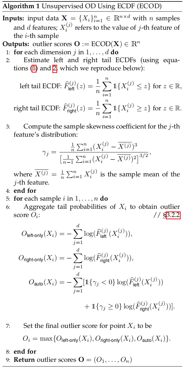
- First, we compute each dimension’s left- and right-tail ECDFs as given in equations (1) and (2).
- For every point \(X_i\) , we aggregate its tail probabilities \(\widehat{F}_{left}^{(j)}(x^{(j)})\) and \(\widehat{F}_{right}^{(j)}(x^{(j)})\) to come up with a final outlier score \(O_i\in[0,\infty)\) ; higher means more likely to be an outlier
Aggregating Outlier Scores
Our aggregation step uses the skewness of a dimension’s distribution to automatically select whether we use the left or the right tail probability for a dimension.
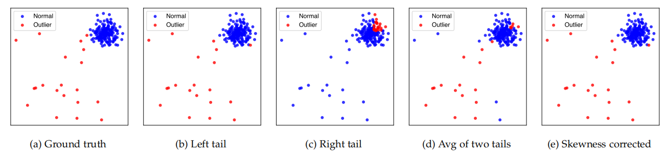
Fig. 1: An illustration of how using different tail probabilities affect the results. The leftmost column are plots of the ground truth, the second column are the result if left tail probabilities are used. The middle column corresponds to outlier detection if right tail probabilities are used, followed by using the average of both tail probabilities in the fourth column and skewness corrected tail probabilities (SC) in the rightmost column (which shows the best result)
In this example, both marginals of \(X_1\) and \(X_2\) skew negatively (i.e., the left tail is longer and the mass of the distribution is concentrated on the right).It makes sense to use the left tail probabilities.
The sample skewness coefficient of dimension j can be calculated as below
where \(\overline{X^{(j)}}=\frac{1}{n}\sum_{i=1}^nX_i^{(j)}\).
When \(\gamma_j < 0\), we can thus consider points in the left tail to be more outlying. When \(\gamma > 0\), we instead consider points in the right tail to be more outlying.
Final aggregation step
We use whichever negative log probability score is highest as the final outlier score $O_i $for point \(X_i\)
pseudocode
Properties of ECOD
-
Interpretable
let \(O_i(j)\) be the dimensional outlier score for dimension \(j\) of \(X_i\) , and using fact that the log function is monotonic, we can see that it represents the degree of outlyingness of dimension \(j\)
Dimensional Outlier Graph
Dataset : Breast Cancer Wisconsin Dataset
The data used has 369 samples, with 9 features listed below, and two outcome classes (benign and malignant).
Features are scored on a scale of 1-10, and are (1) Clump Thickness, (2) Uniformity of Cell Size, (3) Uniformity of Cell Shape, (4) Marginal Adhesion, (5) Single Epithelial Cell Size, (6) Bare Nuclei, (7) Bland Chromatin, (8) Normal Nucleoli and (9) Mitoses.
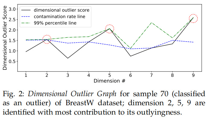
For each of dimension \(j\) (9 dimensions in total) of the \(i\)-th data point, we plot \(O(X_i^{(j)})\), the dimensional outlier score in black.
We also plot the 99th percentile band in green as a reference line
In the analysis below, we plot the Dimensional Outlier Graph for 70-th sample (i = 70), which is malignant (outlier) and has been successfully classified by ECOD.
We see that for dimension/feature 2, 5 and 9, the dimensional outlier scores have “touched” the 99th percentile band, while all other features remain below the contamination rate band. This suggests that this point is likely an outlier because it is extremely non-uniform in size (dim. 2), has a large single epithelial cell size (dim. 5), and is more likely to reproduce via mitosis rather than meiosis (dim. 9).
-
ECOD has \(\mathcal{O}(nd)\) time and space complexity.
In the estimation steps (Section 3.2.1), computing ECDF for all \(d\) dimensions using n samples leads to \(\mathcal{O}(nd)\) time and space complexity.
In the aggregation steps (Section 3.2.2), tail probability calculation and aggregation also lead to \(\mathcal{O}(nd)\) time and space complexity.
阅读的时候想不出 \(\mathcal{O}(nd)\) 的方法实现,然后翻阅源码的时候发现,作者在实际实现的时候,对每个维度进行了
x.sort排序,然后再使用np.searchsorted函数查找当前样本在当前维度中的位置。np.searchsorted的文档中写明是使用Binary Search进行查找。所以计算ECDF的复杂度是 \(\mathcal{O}(ndlogn)\) -
Acceleration by Distributed Learning
Since ECOD estimates each dimension independently, it is suited for distributed learning acceleration with multiple workers.
EMPIRICAL EVALUATION
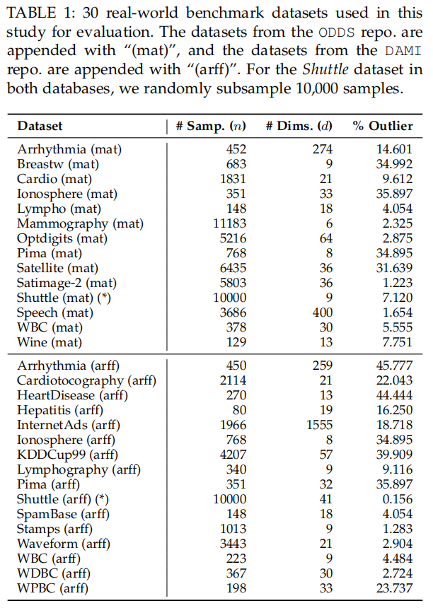
Dataset
Other Outlier Detectors
Performance is evaluated by taking the average score of 10 independent trials using area under the receiver operating characteristic (ROC) and average precision (AP)
We report both the raw comparison results and the critical difference (CD) plots to show statistical difference [55], [56], where it visualize the statistical comparison by Wilcoxon signed-rank test with Holm’s correction.
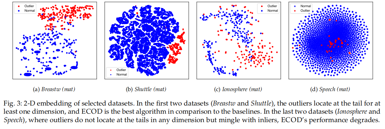
We compare the performance of ECOD with 11 leading outlier detectors.
Specifically, the 11 competitors are AngleBased Outlier Detection (ABOD) [57], Clustering-Based Local Outlier Factor (CBLOF) [40], Histogram-based Outlier Score (HBOS) [30], Isolation Forest (IForest) [17], k Nearest Neighbors (KNN) [15], Lightweight On-line Detector of Anomalies (LODA) [58], Local Outlier Factor(LOF) [34], Locally Selective Combination in Parallel Outlier Ensembles (LSCP) [18], One-Class Support Vector Machines (OCSVM) [16], PCA-based outlier detector (PCA) [59], and Scalable Unsupervised Outlier Detection (SUOD) [21].
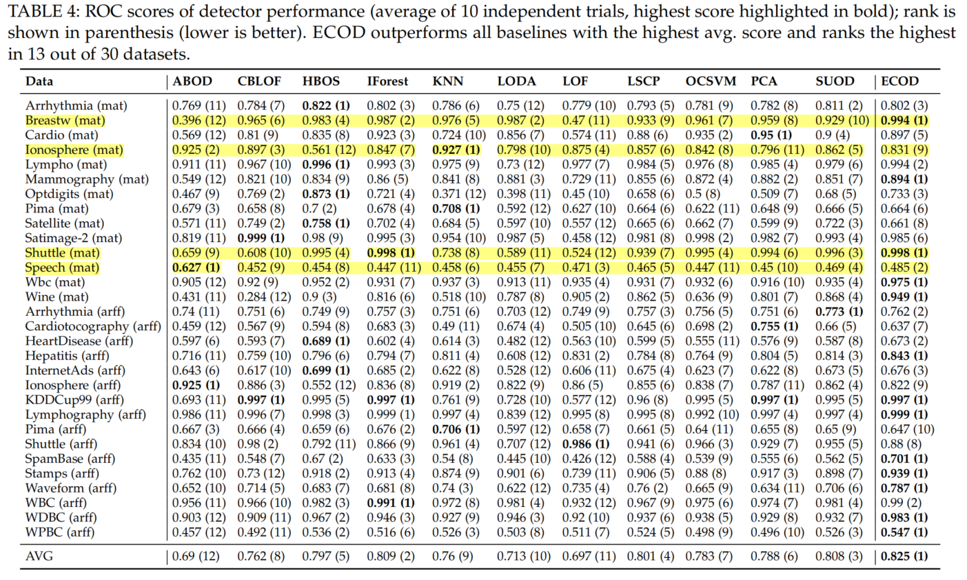
The Effect of Using Different Tails with ECOD
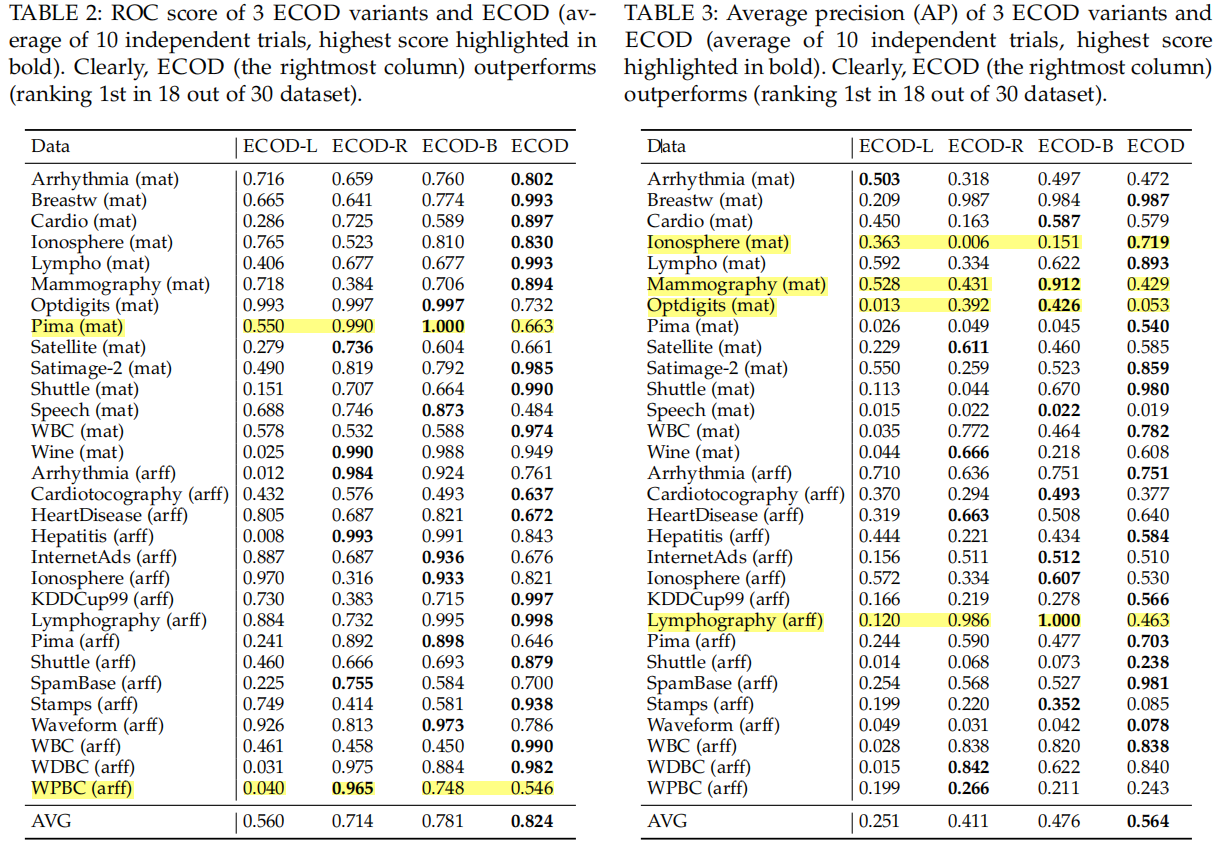
The proposed ECOD achieves the best performance
Its superiority can be credited to the automatic selection of tail probabilities by the skewness of the underlying datasets。
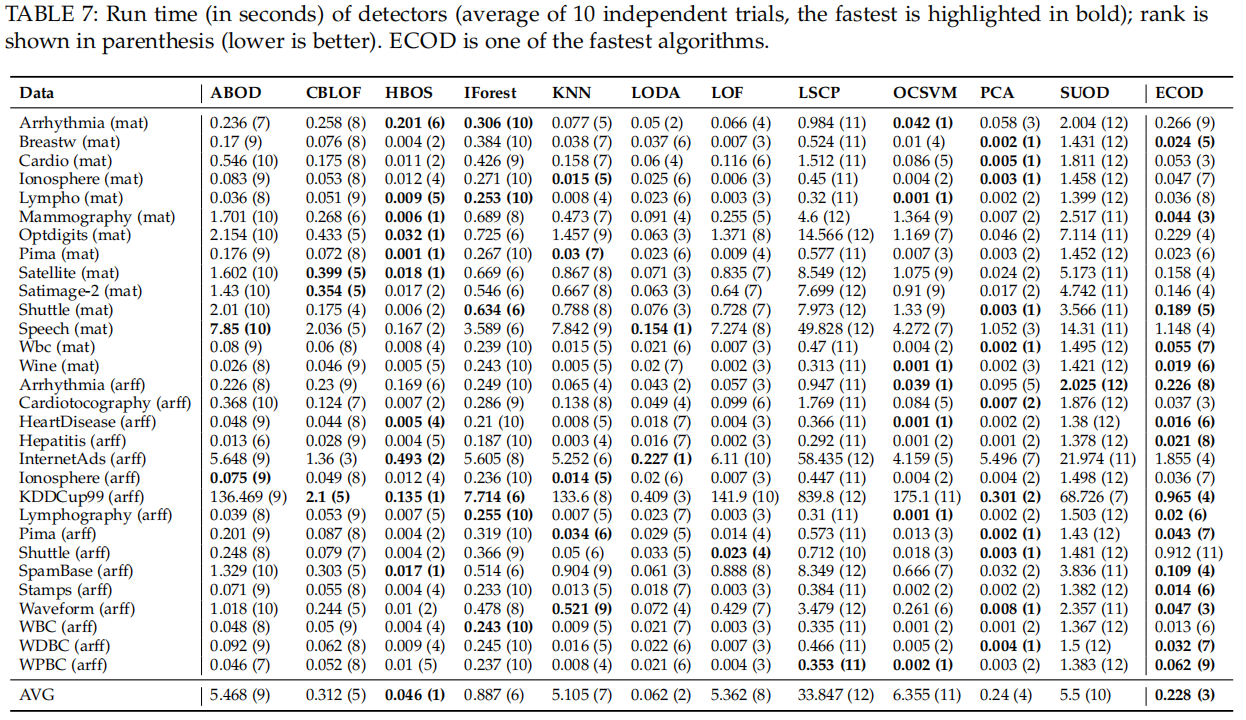
Performance Comparison with Baselines
Of the 30 datasets in Table 1, ECOD scores the highest in terms of ROC (see Table 4). It achieves an average ROC score of 0.825, which is 2% higher than the second best alternative—iForest
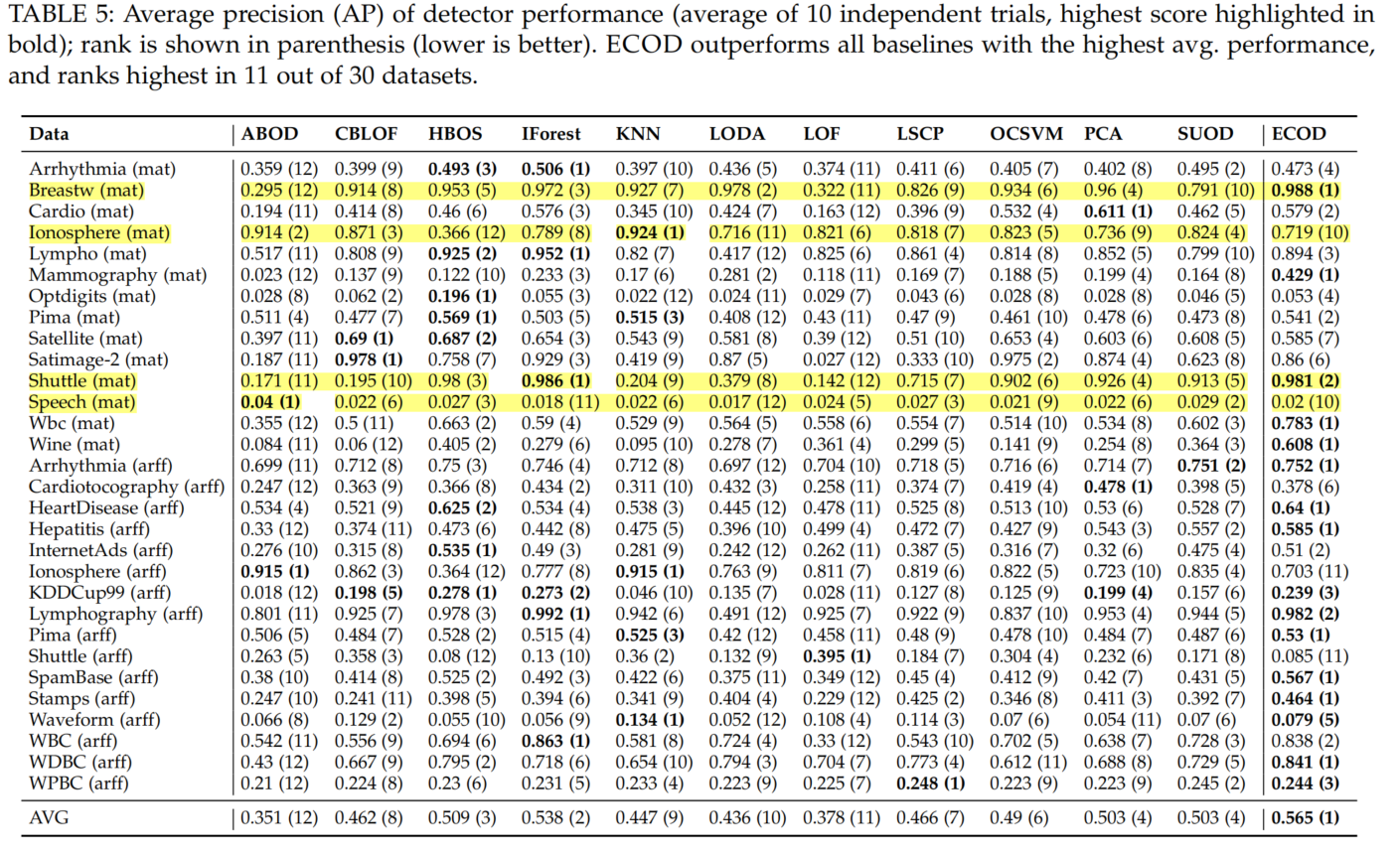
Similarly, Table 5 shows that ECOD is also superior to the baselines regarding AP. Of the 12 OD methods, ECOD achieves an average AP score of 0.565, which bring 5% improvement over the second place—iForest. Additionally, ECOD ranks first in 12 out of 30 datasets, and ranks in the top three places on 20 datasets
Case Study
The visualization suggests that when outliers locates at the tails in at least some dimensions, ECOD could accurate capture them.
However, its performance degrades when outliers are well mingled with normal points (Fig. 3, subfigure c) or hidden in the middle of normal points regarding all dimensions (Fig. 3, subfigure d).
We want to point out that it is unlikely that an outlier resembles normal points in all dimensions, and this explains why ECOD could consistently work for most of the datasets.
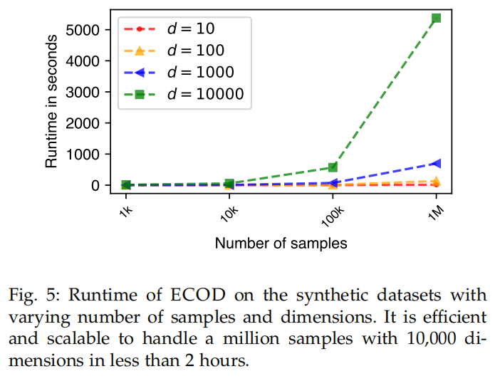
Runtime Efficiency and Scalability
Intuitively, ECOD’s efficiency is attributed to the feature independence assumption.
ECOD is also a scalable algorithm that suits high dimensional settings.
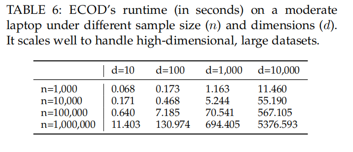
Additionally, ECOD requires no re-training fit new data points with relatively large data samples if no data shift is assumed
- Distribution Unsupervised Cumulative Detection Empiricaldistribution unsupervised cumulative detection distribution detection anomaly论文 discrimination distribution detection anomaly cumulative empirical understanding distillation knowledge empirical minimization empirical beyond mixup self-supervised transformers supervised empirical cumulative特性abap lock 前端cumulative领域layout