1 简单说明
这个文章是讲基于能量意识的动态用户选择, 在hfl的框架下。 因为边缘服务器到客户端这个层级存在着一些选择的关系。
发表在wcnc,一个c类会议上。
2 摘要
Abstract-Federated learning (FL) has become a promising solution to train a shared model without exchanging local training samples. However, in the traditional cloud-based FL framework, clients suffer from limited energy budget and generate excessive communication overhead on the backbone network. These drawbacks motivate us to propose an energy-aware hierarchical federated learning framework in which the edge servers assist the cloud server to migrate the local models from the clients. Then a joint local computing power control and client association problem is formulated in order to minimize the training loss and the training latency simultaneously under the long-term energy constraints. To solve the problem, we recast it based on the general Lyapunov optimization framework with the instantaneous energy budget. We then propose a heuristic algorithm, which takes the importance of local updates into account, to achieve a suboptimal solution in polynomial time. Numerical results demonstrate that the proposed algorithm can reduce the training latency compared to the scheme with greedy client association and myopic energy control, and improve the learning performance compared to the scheme in which the associated clients transmit their local models with the maximal power.
摘要联合学习(FL)已成为一种很有前途的解决方案,可以在不交换局部训练样本的情况下训练共享模型。然而,在传统的基于云的FL框架中,客户端的能源预算有限,并在骨干网络上产生过多的通信开销。这些缺点促使我们提出一种能量感知的分层联合学习框架,其中边缘服务器帮助云服务器从客户端迁移本地模型。然后,为了在长期能量约束下同时最小化训练损失和训练延迟,提出了一个联合的本地计算能力控制和客户端关联问题。为了解决这个问题,我们基于具有瞬时能量预算的一般李雅普诺夫优化框架对其进行了重新定义。然后,我们提出了一种启发式算法,该算法考虑了局部更新的重要性,以在多项式时间内实现次优解。数值结果表明,与贪婪客户端关联和短视能量控制的方案相比,该算法可以减少训练延迟,并与关联客户端以最大功率传输其局部模型的方案相比提高了学习性能。
3 WWW
研究问题: 联邦学习中的能量限制和通信开销问题。
研究目标: 在有限的能量预算内,减少训练损失和加快训练速度(等同于减少通信开销吧)。我的理解。
研究挑战:
-
how to design the client association strategy for higher learning performance and lower training latency。 如何设计具有更高学习性能和更低训练延迟的客户端关联策略。
With limited spectrum resources, associating all the clients to the edge servers can significantly increase the transmission
latency between the clients and the edge servers. Besides, in the scenario where the distribution of the local datasets is non-independent and identically distributed (non-i.i.d.) [11], the clients with different local updates are not equally important to the training. Recently, some works have proposed some scheduling criterions such as gradient variance, model variance, and local loss [12–14] to quantify the importance. As a result, from the perspective of the learning performance, it is better to associate more important clients, that let latency and energy performance might be degraded. Therefore, it is of significant importance to strike a balance. 在频谱资源有限的情况下,将所有客户端关联到边缘服务器可以显著增加传输
客户端和边缘服务器之间的延迟。此外,在局部数据集的分布是非独立和同分布的(非i.i.d.)[11]的情况下,具有不同局部更新的客户端对训练并不同样重要。最近,一些工作提出了一些调度准则,如梯度方差、模型方差和局部损失[12-14]来量化重要性。因此,从学习性能的角度来看,最好关联更重要的客户端,这样可能会降低延迟和能量性能。因此,取得平衡具有重要意义。 -
how to meet the energy budget for the energy-aware clients after multiple* rounds of training? 如何在多轮培训后满足能源意识客户的能源预算。
研究方法: 具有瞬时能量预算的一般李雅普诺夫优化框架,然后提出一个启发式算法,考虑局部更新的重要性。
4 相关工作
-
Hfel: Joint edge association and resource allocation for cost-efficient hierarchical federated edge learning。 这个文章我之前看过,是通过最优化的方法来实现资源分配最后达到精度和成本的平衡。 也算是一个提出hfl的文章。
-
Client-edge-cloud hierarchical federated learning: 又是这篇icc的文章。
-
Federated-learning enabled intelligent fog radio access networks: Fundamental theory, key techniques, and future trends。 这是一个综述,里面好像也介绍了hfl的框架。
5 主要内容
-
系统图毫无营养,就不放了。
-
有K个客户端, S个边缘服务器, client \(k\) in the \(j\)-th iteration in round \(t\) as \(\boldsymbol{\theta}_{k, j}(t)\), to the edge servers, we define the client association strategy as \(\mathcal{A}(t)=\left\{a_{k, s}(t) \mid k \in \mathcal{K}, s \in \mathcal{S}\right\}\), where \(a_{k, s}(t)\) is the client association strategy of client \(k\). Specifically, \(a_{k, s}(t)=1\) indicates that client \(k\) uploads its local model updates to edge。
Case 1: \(j \mid \kappa_1 \neq 0\). The \(\boldsymbol{\theta}_{k, j}(t)\) is updated by local computation: \(\boldsymbol{\theta}_{k, j}(t)=\boldsymbol{\theta}_{k, j-1}(t)-\lambda \nabla F_k\left(\boldsymbol{\theta}_{k, j-1}(t)\right)\), where \(\lambda>0\) is learning rate.
Case 2: \(j \mid \kappa_1=0\) and \(j \mid \kappa_1 \kappa_2 \neq 0\). The \(\boldsymbol{\theta}_{k, j}(t)\) is updated by performing the edge model aggregation on server \(s\) :
\[\boldsymbol{\theta}_{k, j}(t)=\frac{\sum_{i \in \mathcal{K}_s(t)} D_i\left[\boldsymbol{\theta}_{i, j-1}(t)-\nabla F_i\left(\boldsymbol{\theta}_{i, j-1}(t)\right)\right]}{\sum_{i \in \mathcal{K}_s(t)} D_i} . \]Case 3: \(j \mid \kappa_1 \kappa_2=0\). The \(\theta_{k, j}(t)\) is updated by performing the global model aggregation on the cloud server:
\[\boldsymbol{\theta}_{k, j}(t)=\frac{\sum_{i \in \mathcal{Q}(t)} D_i\left[\boldsymbol{\theta}_{i, j-1}(t)-\lambda \nabla F_i\left(\boldsymbol{\theta}_{i, j-1}(t)\right)\right]}{\sum_{i \in \mathcal{O}(t)} D_i} . \]
这3个情况,就是时候进行本地更新,什么时候进行边缘聚合,什么时候进行全局聚合。
- 接下来是计算时间的计算。
然后是能量消耗:
然后是通信时间的计算:
然后居然还有通信的能量损耗,这是我第一次看到,之前的很多论文好像都不说的。
模型分发时间:
边缘服务器上传到云服务器的时间:
于是每轮训练时间的延迟就可以表示为:
然后根据每个client自己计算出的重要度,来评价每个客户端的质量:
Definition 1: In round \(t\), given \(\boldsymbol{\theta}(t)\), the importance of local model updates of client \(k\) is denoted as
这里指数部分,我觉得应该加上一个负号,这样才是正确的。
然后最终的问题形式化:
这里要决策的变量有2个: 1个是a就是用户管理,一个是f,就是频率和工作能力分配。 这个问题显然还是难以解决。 幸运的是,基于李雅普诺夫优化工具[17],这个问题可以通过瞬时能量预算和信道信息来解决。
We first construct a virtual energy queue \(H_k(t)\) to capture the queue dynamics of the energy consumption, which is denoted as \(H_k(t+1)=\left[H_k(t)-\bar{E}_k+E_k(t)\right]^{+}\).
gpt给的解释:
- 这个公式描述了一个虚拟能量队列\(H_k(t)\)的动态行为。队列的状态在每个时间步骤\(t\)都会进行更新。这个队列可能被用于跟踪和管理一个系统(例如一个无线通信系统)的能量消耗。在这个公式中,\(H_k(t)\)表示在时间\(t\)时刻的能量队列状态。\(\bar{E}_k\)表示的可能是在每个时间步骤中消耗的固定能量量,而\(E_k(t)\)则表示在时间\(t\)时刻获得或生成的能量量。\(H_k(t+1)\)表示在时间\(t+1\)时刻的能量队列状态,它是由在时间\(t\)时刻的能量队列状态、固定能量消耗量以及在时间\(t\)时刻获得的能量量共同决定的。这个公式中的\([\cdot]^+\)表示取正部分的操作,也就是说如果\(H_k(t)-\bar{E}_k+E_k(t)\)的结果为负,那么\(H_k(t+1)\)就将被设为0,这意味着能量队列不能有负的能量值。总的来说,这个公式描述了一个系统如何在每个时间步骤中更新其能量队列的状态,以管理其能量消耗。
但是为什么是减去\(\bar{E}_k\)呢,每次消耗难道有这么多能量? 不懂啊。。。。
We then define the Lyapunov function as a scalar metric of queue congestion, i.e., \(Q(t)=\frac{1}{2} \sum_{k=1}^K H_k^2(t)\), where \(\mathcal{H} (t)= { H_k(t) k=1, \ldots, K}\) is the combined matrix of all virtual queues. Then the one-round Lyapunov drift of \(Q(t)\) is defined as \(\Delta_1(t)=Q(t+1)-Q(t)\). In round \(t\), the underlying objective of the proposed resource allocation and client association strategy based on the general Lyapunov optimization framework is to maximum an infimum bound on the drift-plus-penalty expression, which is expressed as
where \(\eta(t)=\sum_{k \in \mathcal{K}} \sum_{s \in \mathcal{S}} a_{k, s}(t) \alpha_k(\boldsymbol{\theta}(t))-T^{\mathrm{r}}(t)\), and \(V>\) 0 is a parameter to control the tradeoff between the energy consumption and the optimal value of the objective function.
gpt给出的解释:
你描述的是一个基于 Lyapunov 优化框架的资源分配和客户关联策略。让我们一步步地解析这段描述。
首先,你定义了一个 Lyapunov 函数 \(Q(t)\),它是队列拥塞的标量度量,通过计算所有虚拟能量队列 \(H_k(t)\) 的平方和的一半来得到。这个函数可以用来衡量系统在时间 \(t\) 的拥塞程度。
然后,你定义了一个一轮的 Lyapunov 漂移 \(\Delta_1(t)\),它是在一轮过后 Lyapunov 函数的变化量,即 \(Q(t+1)-Q(t)\)。
在每一轮 \(t\),你提出的资源分配和客户关联策略的目标是最大化漂移加惩罚项表达式的下确界,这个表达式为 \(V \eta(t)-\Delta_1(t)\)。
其中,\(\eta(t)\) 是一个在时间 \(t\) 的表达式,它是关于 \(a_{k, s}(t)\) 和 \(\alpha_k(\boldsymbol{\theta}(t))\) 的函数,减去 \(T^{\mathrm{r}}(t)\)。这可能是某种系统性能度量,取决于 \(a_{k, s}(t)\)、\(\alpha_k(\boldsymbol{\theta}(t))\) 和 \(T^{\mathrm{r}}(t)\) 的具体含义。
\(V\) 是一个大于 0 的参数,用于控制能量消耗和目标函数最优值之间的权衡。根据 \(V\) 的选择,我们可以在系统性能(由 \(\eta(t)\) 表达)和能量消耗(由 \(\Delta_1(t)\) 表达)之间进行权衡。
总的来说,你描述的是一个基于 Lyapunov 优化的策略,该策略在每一轮中最大化一个漂移加惩罚项表达式的下确界,以此来平衡系统性能和能量消耗的权衡。
接下来引理1就给出下界了:
Lemma 1. Assume that \(H_k(1)=0, \forall k \in \mathcal{K}\). We define \(E^{\max }=\max _{k \in \mathcal{K}} E_k(t), \forall t\) and \(\bar{E}^{\text {min }}=\min _{k \in \mathcal{K}} \bar{E}*k\). Then the drift-plus-penalty satisfies:
where \(\beta\) is a finite constant and satisfies \(\beta \geq \frac{1}{2} \sum*{k=1}^K\left(E^{\max }-\right.\) \(\left.\bar{E}^{\min }\right)^2\).
gpt给的解释:
这个引理(Lemma 1)提供了一个关于漂移加惩罚项表达式 \(V \eta(t) - \Delta_1(t)\) 下界的结果。
假设你的所有虚拟能量队列在初始时刻都为空(即 \(H_k(1) = 0\),对所有的 \(k \in \mathcal{K}\)),你定义了 \(E^{\max}\) 为所有时间步骤中的最大能量生成值,\(\bar{E}^{\text {min}}\) 为所有能量消耗的最小值。
然后,你证明了漂移加惩罚项表达式的下界为:
其中 \(\beta\) 是一个有限常数,满足
这个引理的关键是它提供了一个关于漂移加惩罚项表达式下界的封闭形式,这使得我们能更好地理解和控制这个表达式。这个下界被 \(V \eta(t)\),一个关于系统性能度量的项,以及一个关于能量队列和能量消耗的项所控制。这样的结果可能在设计和分析基于 Lyapunov 优化的策略时非常有用。
然后只要右侧尽量变大就可以了。 于是问题被重新定义为:
但是这个问题仍旧不可解。 所以接下来要设计一个低时间复杂度的算法。
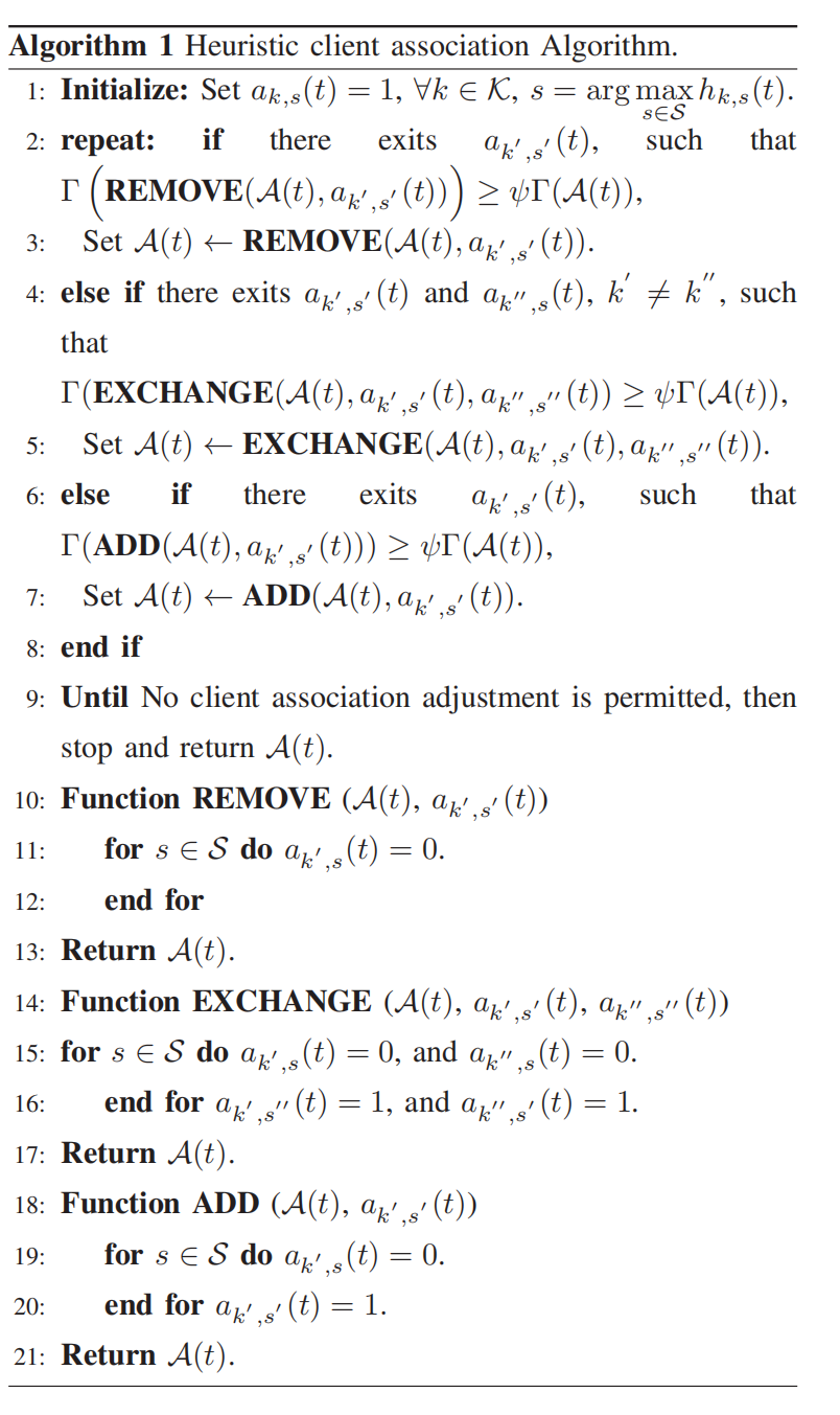
接下来的操作就开始魔幻了,先求解了f的设计,然后用一个类似联盟博弈的方法求解a,提出3种操作,一个是交换,一个是加入,一个离开。
6 实验部分
实验设置:
-
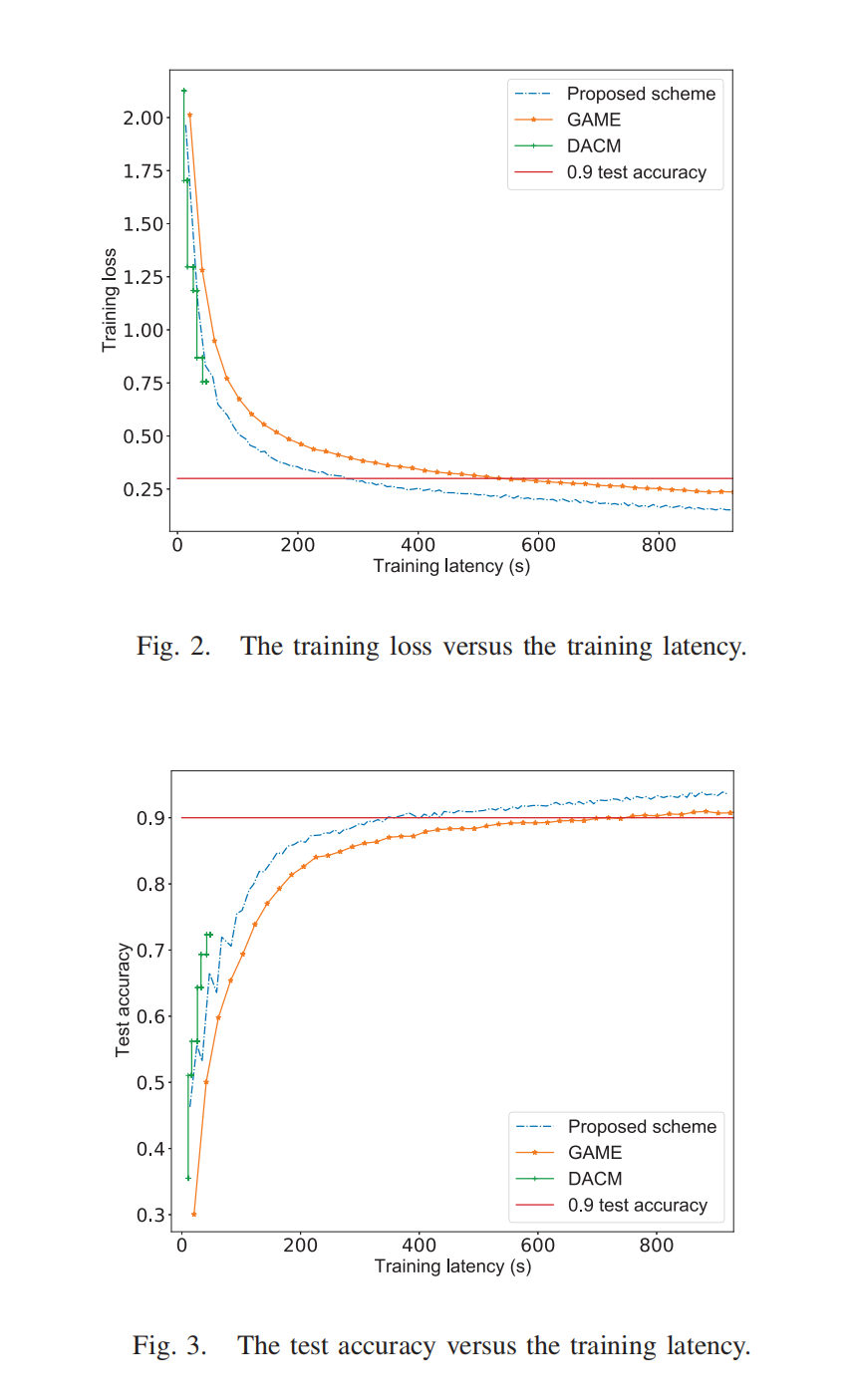
Unless otherwise specified, we consider a system where \(K=50\) clients and \(S=5\) edge servers are uniformly deployed in a area of size \(500 \mathrm{~m} \times 500 \mathrm{~m}\) with a cloud server at its center. The path loss model is given as \(L[\mathrm{~dB}]=\) \(128.1+37.6 \log _{10} d_{[\mathrm{km}]}\), and the standard deviation of the lognormal shadowing fading is \(8 \mathrm{~dB}\) [18]. The total bandwidth is \(B=40 \mathrm{MHz}\), and the spectral density of the noise is \(N_0=-174 \mathrm{dBm} / \mathrm{Hz}\). Parameter \(C_k\) is uniformly distributed in \([1,3] \times 10^4\) cycles/sample. Model size \(M=1\) Mbit. To simplify, we choose an equal transmit power \(p_1(t)=\) \(\ldots=p_K(t)=20 \mathrm{dBm}\), an equal local computing power budget \(f_1^{\max }(t)=\ldots=f_K^{\max }(t)=2.5 \mathrm{GHz}\), and an equal energy budget \(\bar{E}_1=\ldots=\bar{E}_K=0.05 \mathrm{~J}\). Besides, we set the coefficients \(\varrho=10^{-28}, \rho=0.5\), and \(V=0.01\). For the learning model, each client trains a multilayer perceptron model in the well-known dataset MNIST for classification, which consists of 10 categories ranging from digit " 0 " to " 9 ". We sort all training samples according to their digit labels, and assign clients with 500 training samples with only two types of digits [12]. The number of training rounds \(T=100\). In each training round, \(\kappa_1=5\) and \(\kappa_2=10\) [10]. We apply a standard multilayer perceptron model for local computation which has one hidden layer of 64 hidden nodes, We apply a standard multilayer perceptron (MLP) model for local model updates which has one hidden layer of 64 hidden nodes, and use ReLU activation. The MLP model has 50,890 weights. In addition, in this paper, we compare the performance of the proposed algorithm against the following baselines 1) Greedy client association with monotonous energy control (GAME): All the clients are selected and greedily associated to the edge servers that have the highest channel gains. Then all the clients make the local computing power control while satisfying the instantaneous energy budget, i.e., \(E_k(t)=\bar{E}_k, \forall t \in \mathcal{T}\)。
这里设计了一些常用的参数,50个客户,5个边缘服务器,然后信噪比,功率,带宽,关键系数。 本地轮次和边缘轮次,用了mnist数据和mlp模型。
几个baseline:
- 贪心,每个客户都贪心的选择有最高的信噪比的,每个刚好把能量用完。
- Latency-aware client association with maximal local computing power (DACM): Based on the proposed client association algorithm, all associated clients perform the local training with their maximal local computing power。 具有最大本地计算能力的延迟感知客户端关联(DACM):基于所提出的客户端关联算法,所有关联的客户端都以其最大本地计算力进行本地训练。
-
实验图就2个,太简单了,损失和精度,本质上是一样的东西。
- Energy-Aware Hierarchical Association Federated Learningenergy-aware hierarchical association federated federated learning 005 heterogeneous federated learning yourself genome-wide association overview learning healthcare federated learning会议 energy-aware hierarchical federated transformer hierarchical shifted windows association