https://developer.ibm.com/articles/cc-cognitive-neural-networks-deep-dive/
By M. Tim Jones, Published July 23, 2017
Neural networks have been around for more than 70 years, but the introduction of deep learning has raised the bar in image recognition and even learning patterns in unstructured data (such as documents or multimedia). Deep learning is based on fundamental concepts of the perceptron and learning methods like back-propagation. This tutorial implements and works its way through single-layer perceptrons to multilayer networks and configures learning with back-propagation to give you a deeper understanding.
Neural networks are computational models for machine learning that are inspired by the structure of the biological brain. Neural networks are trained from examples rather than being explicitly programmed. Even with limited examples, neural networks can generalize and successfully deal with unseen examples.
Neural networks began with the simple, single-layer perceptrons, but they are now represented by a diverse set of architectures that include multiple layers and even recurrent connections to implement feedback. Let's start with the biological inspiration for neural networks.
Biological inspiration
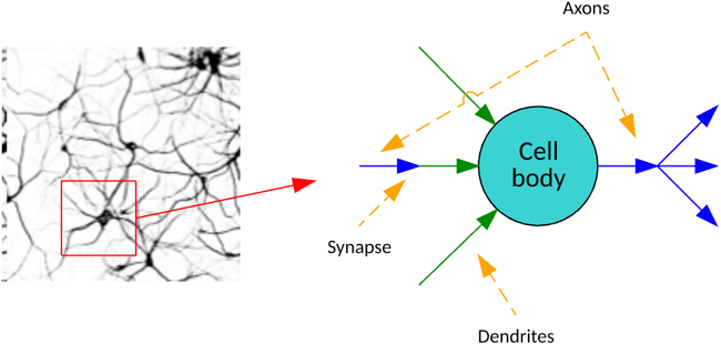
Neural networks represent an information-processing paradigm that is loosely inspired by the human brain. In the brain, neurons are highly connected and communicate chemical signals through synapses between axons and dendrites. The human brain is estimated to have 100 billion neurons, with each neuron connected to up to 10,000 other neurons.
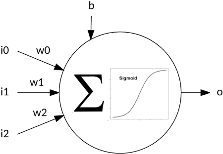
Artificial neural networks communicate signals (numbers) through weights and activation functions (such as sigmoids) that activate neurons. Using a training algorithm, these networks adjust those weights to solve a given problem. The following image illustrates a single perceptron that has three inputs: a weight for each input, an input bias, and an output. The output is calculated from the summation of the input and weight products, including the bias pass through an activation function. I explore the lowly perceptron as a first example before venturing further into back-propagation.
Neural networks today can be sparsely connected, fully connected, recurrent (include cycles), and various other architectures. Let's take a quick tour through the history of neural networks.
A history of neural networks
In the early 1940s, McCulloch and Pitts created a computational model for neural networks that spawned research not only into the brain but also its application to artificial intelligence (AI; see the following image). Later in this decade, Donald Hebb created Hebbian learning, which observed from biology that the synapse between two neurons is strengthened if the two neurons are simultaneously active.
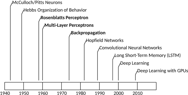
In 1958, Frank Rosenblatt created the perceptron, a simple neural model that could be used to classify data into two sets. However, this model suffered in that it could not correctly classify an exclusive-OR. Marvin Minsky and Seymour Papert exploited this limitation in 1969 in their book Perceptrons in an attempt to return focus to symbolic methods for AI. The result was a decade-long decline in connectionist research funding.
In 1975, Paul Werbos created the back-propagation algorithm, which could successfully train multilayer perceptrons and introduced various new applications of multilayer neural networks. This innovation led to a resurgence in neural network research and further popularized the method to solve real problems.
Since the introduction of back-propagation, neural networks have continued their rise as a key algorithm in machine learning. In recent decades, the introduction of graphical processing units (GPUs) and distributed processing have made it possible to train large neural networks by offloading neural network training and execution to clusters of accelerators. The result was deep learning architectures (convolutional neural networks and long short-term memory [LSTM]), which have greatly expanded the applications of neural networks and the problems they address.
Perceptrons
The perceptron is an example of a simple neural network that can be used for classification through supervised learning. Supervised means that we train the network with examples, and then adjust the weights based on the actual output from the desired output.
Frank Rosenblatt created the first perceptron, simulating first on an IBM® 704 computer, and then later implementing the perceptron as custom hardware (called the Mark 1 Perceptron), with an array of 400 photocells for vision applications. The photocells were randomly connected to neurons, and the weights were implemented as potentiometers (variable resistors) that could be adjusted by attached motors as part of the learning process.
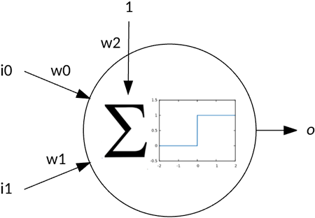
The following image shows a simple perceptron that includes two inputs (with associated weights) and a bias weight. The perceptron operates by summing the products of the inputs and their associated weights, and then applying that result through an activation function. In this example, the activation function is a step function that says that if the output is greater than or equal to 1, then the output is 1 (otherwise, the output is 0).
The simple perceptron could be used to solve linear separable problems, as shown in the following image. In this illustration, a line divides the two classes (the result of a logical OR operation), which can be implemented as a straight line (or decision boundary). That decision boundary is a function of the weights for the inputs and the bias. Both the OR and the AND problems are linearly separable, but the XOR is not (given 1 XOR 1 is 0 and not separable).

Now that you have some insight into the problems perceptrons can solve, let's look at how you "educate" the perceptron through supervised training.
Perceptron learning
Perceptron learning, like many other supervised learning algorithms, follows a simple flow but differs in the way the network is adjusted. Let's look at a general example, and then dig into perceptron learning.
The following figure illustrates the general supervised flow. I first initialize my network (topology is not fixed and initial weights). Then, I iterate by applying a training vector to the network and based on its error (actual versus desired output), I adjust the weights of my neural network to classify this input properly in the future. I then implement a stopping condition (no more errors are found or based on some number of training iterations). When this process is complete, I validate the network with unseen training examples (to see how well it generalizes to unseen input), and then deploy the network into its intended application.
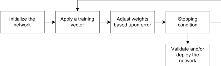
Perceptron learning follows this general flow. I initialize the weights of my network to a random set of values. I then iterate over my training set until I see no further errors. Applying a training vector means applying a training vector to the network and executing the network (feeding that training vector forward to yield an output value). I subtract this output from the desired output (called the error). I use this error, with a small learning rate, to adjust the weight based on the contribution of the input. In other words, the weight is adjusted by the error multiplied by the input (associated with the given weight) multiplied by a small learning rate. This process continues until no more errors occur.
Perceptron example
Let's look at the implementation of this algorithm as applied to the logical OR operation. You can download and experiment with this implementation from GitHub.
In the following code listing, you can see the variable definition. It defines the size of the input vector (ISIZE), the size of the weight vector (ISIZE+1 to account for the bias weight), my small learning rate, a maximum number of iterations, and the types of my input and weight vectors.
In the following code listing, you can see the variable definition. It defines the size of the input vector (ISIZE), the size of the weight vector (ISIZE+1 to account for the bias weight), my small learning rate, a maximum number of iterations, and the types of my input and weight vectors.
#define ISIZE 2
#define WSIZE ( ISIZE + 1 ) // weights + bias
#define LEARNING_RATE  0.1
#define ITERATIONS     10

typedef int ivector[ ISIZE ];
typedef float wvector[ WSIZE ];
wvector weights;
The next code listing shows my network initialization. In this function, I seed the random number generator, and then initialize each weight in the weight vector to a random floating point number between 0 and 1.
void initialize( void )
{
   // Seed the random number generator
   srand( time( NULL ) );

   // Initialize the weights with random values
   for ( int i = 0 ; i </ WSIZE ; i++ )
   {
      weights[ i ] = ( ( float ) rand( ) / ( float ) RAND_MAX );
   }
}
The following code example illustrates the execution of the network. The feedforward function is passed the training vector, which is then used to calculate the output of the neuron (per the equation found in Figure 4). At the end, I apply the step activation function and return the result.
int feedforward( ivector inputs )
{
   int i;
   float sum = 0.0;

   // Calculate inputs  weights
   for ( i = 0 ; i < ISIZE ; i++ )
   {
      sum += weights[ i ]  ( float ) inputs[ i ];
   }

   // Add in the bias
   sum += weights[ i ];

   // Activation function (1 if value >= 1.0).
   return ( sum >= 1.0 ) ? 1 : 0;
}
The final function, train, is shown in the following code listing. In this function, I iterate over the training set, applying the test pattern to the network (through feedforward), and then calculating an error based on the resulting output. Given the error, I adjust each of the three weights based on the learning rate and the contribution of the input. This process stops when no further errors are found (or I exceed the maximum number of iterations).
void train( void )
{
   int iterations = 0;
   int iteration_error = 0;
   int desired_output, output, error;

   // Train the boolean OR set
   ivector test[4] = { { 0, 0 }, { 0, 1 }, { 1, 0 }, { 1, 1 } };

   do
   {
      iteration_error = 0.0;
      for ( int i = 0 ; i < ( sizeof( test ) / sizeof( ivector ) ) ; i++ )
      {
         desired_output = test[ i ][ 0 ] || test[ i ][ 1 ];
         output = feedforward( test[ i ] );
         error = desired_output ‑ output;
         weights[ 0 ] += ( LEARNING_RATE
                           ( ( float ) error  ( float )test[ i ][ 0 ] ) );
         weights[ 1 ] += ( LEARNING_RATE
                           ( ( float ) error  ( float )test[ i ][ 1 ] ) );
         weights[ 2 ] += ( LEARNING_RATE  ( float ) error );
         iteration_error += ( error  error );
      }
   } while ( ( iteration_error > 0.0 ) && ( iterations++ < ITERATIONS ) );
   return;
}
Finally, in the following code, you can see sample output for this simple example. In this example, the training required three iterations to learn the OR operation (the value in parentheses is the desired output). The final weights are also shown, including the bias.
$ ./perceptron
Iteration 0
0 or 0 = 0 (0)
0 or 1 = 0 (1)
1 or 0 = 0 (1)
1 or 1 = 0 (1)
Iteration error 3

Iteration 1
0 or 0 = 0 (0)
0 or 1 = 0 (1)
1 or 0 = 0 (1)
1 or 1 = 1 (1)
Iteration error 2

Iteration 2
0 or 0 = 0 (0)
0 or 1 = 1 (1)
1 or 0 = 1 (1)
1 or 1 = 1 (1)
Iteration error 0

Final weights 0.374629 0.417000 bias 0.700291
In approximately 65 lines of C, you can implement perceptron learning. See the GitHub site for the full source.
Multilayer networks
Adding layers of neurons increased the complexity of the problems that can be applied to neural networks. This same principle is being applied today in deep learning, as more layers (the depth) are added with some new ideas to solve even more complex and varied problems (see the following image for an example network with an input layer, a hidden layer, and an output layer).
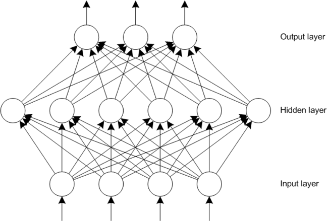
Hidden layers are important because they provide the ability to extract features from the input layer. But, the number of hidden layers (and neurons in each layer) is a function of the problem at hand. If a network includes too many neurons in a hidden layer, it can overfit and simply memorize the input patterns, which limits the network's ability to generalize. Too few neurons in the hidden layer can result in the network being unable to represent the input-space features and also limit the networks' ability to generalize. In general, the smaller the network (fewer neurons and weights), the better the network.
The process of executing a network with multiple layers is similar to the perceptron model. Inputs are fed through weights into the hidden layer, and hidden layer outputs are fed through weights into the output layer. The output can represent multiple features or as I demonstrate in the next section, a single feature in a winner-takes-all system (where the largest output neuron is the winner).
Back-propagation
The back-propagation algorithm has a long history. It was introduced in the 1970s, but its potential wasn't realized until the 1980s. More than 30 years later, the back-propagation algorithm remains a popular technique for neural network training. What makes back-propagation so important is that it's both fast and efficient. Back-propagation gets its name from its process: the backward propagation of errors within a network.
Back-propagation follows a similar training flow to that shown in the Perceptron learning section. An input vector is applied to the network and propagated forward from the input layer to the hidden layer, and then to the output layer. An error value is then calculated by using the desired output and the actual output for each output neuron in the network. The error value is propagated backward through the weights of the network beginning with the output neurons through the hidden layer and to the input layer (as a function of the contribution of the error).
This process organizes the network such that the hidden layer recognizes features in the input space. The output layer uses the hidden layer features to arrive at a solution. As you'll see in the example implementation, the back-propagation algorithm is not computationally expensive in terms of modern computing, but GPUs have made it possible to build massive networks within clusters of GPU-based systems that are capable of incredible tasks, such as object recognition.
Back-propagation example
Now, let's look at a simple implementation of back-propagation. In this example, I train a simple network by using Fisher's Iris flower data set. This data set includes four measurements representing the length and width of flower petals and sepals within three species of the iris flower (setosa, virginica, and versicolor). The goal is to train the network so that it can successfully classify an iris based on its four measured features. You can download and try this code for yourself from GitHub.
The following code listing shows my variable definition. I define the size of my layers with the input layer defining my four features, a hidden layer containing 25 neurons, and an output layer representing a winner-takes-all representation of the three iris species. Three arrays define the values of each neuron (inputs, hidden, and outputs), and the weights are represented by two multidimensional arrays that include biases. A small learning rate is also provided.
#define INP_NEURONS    4
#define HID_NEURONS   25
#define OUT_NEURONS    3

#define LEARNING_RATE 0.05

// Neuron cell values
double inputs[ INP_NEURONS+1 ];
double hidden[ HID_NEURONS+1 ];
double outputs[ OUT_NEURONS ];

// Weight values
double weights_hidden_input[ HID_NEURONS ][ INP_NEURONS+1 ];
double weights_output_hidden[ OUT_NEURONS ][ HID_NEURONS+1 ];
In the next code example, you can see the representation of my training data set, which consists of individual training samples (of the four features) with its species classification (into 1 of 3 output nodes). The entire data set contains 150 samples, so I provide an abridged version here.
// Test dataset with desired outputs (in a winner‑takes‑all fashion).
typedef struct dataset_s
{
   double inputs[ INP_NEURONS  ];
   double output[ OUT_NEURONS ];
} dataset_t;

dataset_t dataset[ ] = {
// Sepal Length, Sepal Width, Petal Length, Petal Width
                          // Iris‑setosa
{ { 5.1, 3.5, 1.4, 0.2 }, { 1.0, 0.0, 0.0 } },
{ { 4.9, 3.0, 1.4, 0.2 }, { 1.0, 0.0, 0.0 } },
…
                          // Iris‑versicolor
{ { 7.0, 3.2, 4.7, 1.4 }, { 0.0, 1.0, 0.0 } },
{ { 6.4, 3.2, 4.5, 1.5 }, { 0.0, 1.0, 0.0 } },
…
                         // Iris‑virginica
{ { 6.3, 3.3, 6.0, 2.5 }, { 0.0, 0.0, 1.0 } },
{ { 5.8, 2.7, 5.1, 1.9 }, { 0.0, 0.0, 1.0 } },
…
The code to execute a network is provided in the following code listing. You can split this listing into three parts. The first takes the input neurons and calculates the outputs of the hidden layer neurons. The next section takes the hidden neurons and calculates the outputs of the output layer neurons. This is the entire process of feeding the inputs forward through the network (each layer using a sigmoidal activation function). When the outputs have been calculated, the output neurons are iterated, and the largest value is selected in a winner-takes-all fashion. This output neuron is then returned as the solution.
// Given the test input, feed forward to the output.
int NN_Feed_Forward( void )
{
   int i, j, best;
   double max;

   // Calculate hidden layer outputs
   for ( i = 0 ; i < HID_NEURONS ; i++ )
   {
      hidden[ i ] = 0.0;

      for ( j = 0 ; j < INP_NEURONS+1; j++ )
      {
         hidden[ i ] +=
            ( weights_hidden_input[ i ][ j ]  inputs[ j ] );
      }
      hidden[ i ] = sigmoid( hidden[ i ] );
   }

   // Calculate output layer outputs
   for ( i = 0 ; i < OUT_NEURONS ; i++ )
   {
      outputs[ i ] = 0.0;
      for ( j = 0 ; j < HID_NEURONS+1 ; j++ )
      {
         outputs[ i ] +=
            ( weights_output_hidden[ i ][ j ]  hidden[ j ] );
      }
      outputs[ i ] = sigmoid( outputs[ i ] );
   }

   // Perform winner‑takes‑all for the network.
   best = 0;
   max = outputs[ 0 ];

   for ( i = 1 ; i < OUT_NEURONS ; i++ )
   {
      if ( outputs[ i ] > max )
      {
         best = i;
         max = outputs[ i ];
      }
   }

   return best;
}
Learning is implemented using back-propagation, as shown in the following code example. This is implemented in four parts. First, I calculate the error of the output nodes. Each is calculated independently based on its error (from desired output) and the derivative of the sigmoid function. The error of the hidden layer neurons is then calculated based on their contribution to the output error. The last two parts are then to apply the errors to the output and hidden layers, with a learning rate to minimize the overall change and allow it to be tuned over some number of iterations.
This process implements gradient descent search, as the error is minimized in the neuron outputs (the gradient shows the largest rate of increase of the error, so I move in the opposite direction of the gradient).
// Given a classification, backpropagate the error through the weights.
void NN_Backpropagate( int test )
{
   int out, hid, inp;

   double err_out[ OUT_NEURONS ];
   double err_hid[ HID_NEURONS ];

   // Calculate output node error
   for ( out = 0 ; out < OUT_NEURONS ; out++ )
   {
      err_out[ out ] =
         ( ( double ) dataset[ test ].output[ out ] ‑ outputs[ out ] )
            sigmoid_d( outputs[ out ] );
   }

   // Calculate the hidden node error
   for ( hid = 0 ; hid < HID_NEURONS ; hid++ )
   {
      err_hid[ hid ] = 0.0;
      for ( out = 0 ; out < OUT_NEURONS ; out++ )
      {
         err_hid[ hid ] +=
            err_out[ out ]  weights_output_hidden[ out ][ hid ];
      }
      err_hid[ hid ] = sigmoid_d( hidden[ hid ] );
   }

   // Adjust the hidden to output layer weights
   for ( out = 0 ; out < OUT_NEURONS ; out++ )
   {
      for ( hid = 0 ; hid < HID_NEURONS ; hid++ )
      {
         weights_output_hidden[ out ][ hid ] +=
            LEARNING_RATE  err_out[ out ]  hidden[ hid ];
      }
   }

   // Adjust the input to hidden layer weights
   for ( hid = 0 ; hid < HID_NEURONS ; hid++ )
   {
      for ( inp = 0 ; inp < INP_NEURONS+1 ; inp++ )
      {
         weights_hidden_input[ hid ][ inp ] +=
            LEARNING_RATE  err_hid[ hid ] * inputs[ inp ];
      }
   }
}
In the final part of this implementation, you can see the overall training process. I use some number of iterations as my halting function and simply apply a random test case to the network, and then check the error and back-propagate the error through the weights of the network.
// Train the network from the test vectors.
void NN_Train( int iterations )
{
   int test;

   for ( int i = 0 ; i < iterations ; i++ )
   {
      test = getRand( MAX_TESTS );

      NN_Set_Inputs( test );

      (void)NN_Feed_Forward( );

      NN_Backpropagate( test );
   }

   return;
}
In the sample output below, you can see the result of the back-propagation demonstration. When the network is trained, it takes a random sample of the data set and tests the network against them. What is shown below are those 10 test samples, which are all successfully classified (the output is the output neuron index), and the values that are shown in parentheses are the desired output neuron (the first is index 0, second is index 1, and so on).
$ ./backprop
Test 9 classifed as 0 (1 0 0)
Test 133 classifed as 2 (0 0 1)
Test 78 classifed as 1 (0 1 0)
Test 129 classifed as 2 (0 0 1)
Test 1 classifed as 0 (1 0 0)
Test 59 classifed as 1 (0 1 0)
Test 31 classifed as 0 (1 0 0)
Test 87 classifed as 1 (0 1 0)
Test 122 classifed as 2 (0 0 1)
Test 138 classifed as 2 (0 0 1)
Going further
Neural networks are the dominant force in machine learning today. After their decline, when they failed to meet the unreasonable expectations of their creators, neural networks are today behind the massive momentum in deep learning and new approaches within this field (such as back-propagation through time and LSTM). From the simple models of the 1940s and 1950s (perceptrons) to the breakthroughs of the 1970s and 1980s (back-propagation), these simple models that attempted to mimic the structure of the brain are driving new applications and innovations in AI.
Take a look at Get started with AI to begin your AI journey.
- networks neural BIgdataAIML-IBM-A introduction BIgdataAIMLnetworks neural bigdataaiml-ibm-a introduction bigdataaiml-ibm-a neural-network learning networks neural hello deep-neural-network-driven graph condensation networks neural understanding plasticity networks neural decoupling networks neural depth pre-train learning networks neural convolutional networks neural cnn