原文： https://towardsdatascience.com/3d-data-processing-with-open3d-c3062aadc72e

 

 In this article, I provide a quick walkthrough on how to explore, process and visualize 3D models using Python’s Open3D library — an open-source library for 3D data processing.

You might find this walkthrough helpful if you’re thinking of processing 3D data/models for specific tasks, such as training an AI model for 3D model classification and/or segmentation. 3D models found on the internet (in datasets like ShapeNet) are available in a variety of formats, such as .obj, .glb, .gltf, and so on. Using libraries like Open3D, such models can be easily processed, visualized and converted to other formats, like point clouds, which are easier to understand and interpret.

This article is also available as a Jupyter Notebook for those who wish to follow along and run the code locally. The zip file containing the Jupyter Notebook along with all the other data and assets can be downloaded from the link below.

In this tutorial, I go through the following tasks:

1. Loading and visualizing a 3D model as a mesh
2. Converting the mesh to a point cloud by sampling points
3. Removing hidden points from the point cloud
4. Converting the point cloud to a dataframe
5. Saving the point cloud and dataframe

Let’s start by importing all the necessary libraries:

# Importing open3d and all other necessary libraries.

import open3d as o3d
import os
import copy
import numpy as np
import pandas as pd
from PIL import Image

np.random.seed(42)

# Checking the installed version on open3d.

o3d.__version__
# Open3D version used in this exercise: 0.16.0

Loading and visualizing a 3D model as a mesh

The 3D model can be read as a mesh by running the following lines of code:

# Defining the path to the 3D model file.
mesh_path = "data/3d_model.obj"

# Reading the 3D model file as a 3D mesh using open3d.
mesh = o3d.io.read_triangle_mesh(mesh_path)

To visualize the mesh, run the following lines of code:

# Visualizing the mesh.
draw_geoms_list = [mesh]
o3d.visualization.draw_geometries(draw_geoms_list)

The mesh should open up in a new window and should look like the image below (take note that the mesh opens up as a static image, and not like the animated one shown here). The mesh image can be rotated around as needed using the mouse pointer.

As seen above, the car mesh does not appear like a typical 3D model, and is painted in a uniform grey colour. This is because the mesh does not have any information about normals for the vertices and the surfaces in the 3D model.

What are normals? — The normal vector to a surface at a given point is a vector which is perpendicular to the surface at that point. The normal vector is often simply called the “normal”. To read more on this topic, you can refer to these two links: Normal Vector and Estimating Surface Normals in a PointCloud.

The normals for the 3D mesh above can be estimated by running the following lines of code:

# Computing the normals for the mesh.
mesh.compute_vertex_normals()

# Visualizing the mesh.
draw_geoms_list = [mesh]
o3d.visualization.draw_geometries(draw_geoms_list)

Once visualized, the mesh should now appear as shown in the image below. After computing the normals, the car renders properly and looks like a 3D model.

Let us now create a XYZ coordinate frame to understand the orientation of this car model in the Euclidean space. The XYZ coordinate frame can be overlaid on the 3D mesh above and visualized by running the following lines of code:

# Creating a mesh of the XYZ axes Cartesian coordinates frame.
# This mesh will show the directions in which the X, Y & Z-axes point,
# and can be overlaid on the 3D mesh to visualize its orientation in
# the Euclidean space.
# X-axis : Red arrow
# Y-axis : Green arrow
# Z-axis : Blue arrow
mesh_coord_frame = o3d.geometry.TriangleMesh.create_coordinate_frame(size=5, origin=[0, 0, 0])

# Visualizing the mesh with the coordinate frame to understand the orientation.
draw_geoms_list = [mesh_coord_frame, mesh]
o3d.visualization.draw_geometries(draw_geoms_list)

From the above visualization, we see that this car mesh is oriented as follows:

• Origin of XYZ axes : At the volumetric center of the car model (not seen in the image above as it is inside the car mesh).
• X-axis (Red arrow) : Along the length dimension of the car with positive X-axis pointing towards the hood of the car (not seen in the image above as it is inside the car mesh).
• Y-axis (Green arrow) : Along the height dimension of the car with the positive Y-axis pointing towards the roof of the car.
• Z-axis (Blue arrow) : Along the width dimension of the car with the positive Z-axis pointing towards the right side of the car.

Let us now take a look at what is inside this car model. To do this, we will crop the mesh in the Z-axis and remove the right half of the car (positive Z-axis).

# Cropping the car mesh using its bouding box to remove its right half (positive Z-axis).
bbox = mesh.get_axis_aligned_bounding_box()
bbox_points = np.asarray(bbox.get_box_points())
bbox_points[:, 2] = np.clip(bbox_points[:, 2], a_min=None, a_max=0)
bbox_cropped = o3d.geometry.AxisAlignedBoundingBox.create_from_points(o3d.utility.Vector3dVector(bbox_points))
mesh_cropped = mesh.crop(bbox_cropped)

# Visualizing the cropped mesh.
draw_geoms_list = [mesh_coord_frame, mesh_cropped]
o3d.visualization.draw_geometries(draw_geoms_list)

From the above visualization, we see that this car model has a detailed interior. Now that we have seen what is inside this 3D mesh, we can convert it to a point cloud before removing the “hidden” points which belong to the interior of the car.

Converting the mesh to a point cloud by sampling points

Converting the mesh to a point cloud can be easily done in Open3D by defining the number of points we wish to sample from the mesh.

# Uniformly sampling 100,000 points from the mesh to convert it to a point cloud.
n_pts = 100_000
pcd = mesh.sample_points_uniformly(n_pts)

# Visualizing the point cloud.
draw_geoms_list = [mesh_coord_frame, pcd]
o3d.visualization.draw_geometries(draw_geoms_list)

Take note that the colours in the point cloud above only indicate the position of the points along the Z-axis.

If we were to crop the point cloud exactly like we did for the mesh above, this is what it would look like:

# Cropping the car point cloud using bounding box to remove its right half (positive Z-axis).
pcd_cropped = pcd.crop(bbox_cropped)

# Visualizing the cropped point cloud.
draw_geoms_list = [mesh_coord_frame, pcd_cropped]
o3d.visualization.draw_geometries(draw_geoms_list)

We see in this visualization of the cropped point cloud that it also contains points which belong to the interior of the car model. This is expected as this point cloud was created by uniformly sampling points from the entire mesh. In the next section, we will remove these “hidden” points which belong to the interior of the car and are not on the outer surface of the point cloud.

Removing hidden points from the point cloud

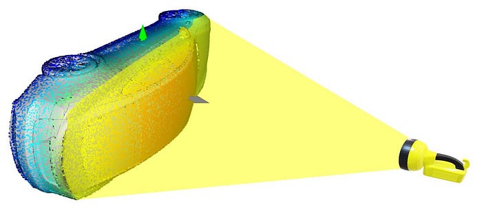
Imagine yourself pointing a light on the right side of the car model. All the points that fall on the right outer surface of the 3D model would be illuminated, while all the other points in the point cloud would not.

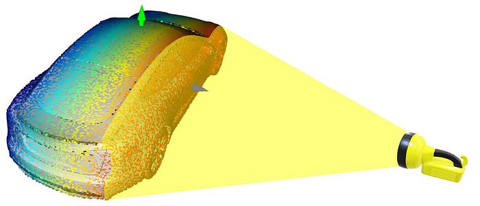
Let us now label these illuminated points as “visible” and all the non-illuminated points as “hidden”. These “hidden” points would also include all the points that belong to the interior of the car.

This operation is known as Hidden Point Removal in Open3D. In order to perform this operation on the point cloud using Open3D, run the following lines of code:

# Defining the camera and radius parameters for the hidden point removal operation.
diameter = np.linalg.norm(np.asarray(pcd.get_min_bound()) - np.asarray(pcd.get_max_bound()))
camera = [0, 0, diameter]
radius = diameter * 100

# Performing the hidden point removal operation on the point cloud using the
# camera and radius parameters defined above.
# The output is a list of indexes of points that are visible.
_, pt_map = pcd.hidden_point_removal(camera, radius)

Using the above output list of indexes of points that are visible, we can colour the visible and hidden points in different colours before visualizing the point cloud.

# Painting all the visible points in the point cloud in blue, and all the hidden points in red.

pcd_visible = pcd.select_by_index(pt_map)
pcd_visible.paint_uniform_color([0, 0, 1])    # Blue points are visible points (to be kept).
print("No. of visible points : ", pcd_visible)

pcd_hidden = pcd.select_by_index(pt_map, invert=True)
pcd_hidden.paint_uniform_color([1, 0, 0])    # Red points are hidden points (to be removed).
print("No. of hidden points : ", pcd_hidden)

# Visualizing the visible (blue) and hidden (red) points in the point cloud.
draw_geoms_list = [mesh_coord_frame, pcd_visible, pcd_hidden]
o3d.visualization.draw_geometries(draw_geoms_list)

From the visualization above, we see how the hidden point removal operation works from a given camera viewpoint. The operation eliminates all the points in the background that are occluded by the points in the foreground from a given camera viewpoint.

To understand this better, we could repeat the same operation again, but this time after rotating the point cloud slightly. Effectively, we’re trying to change the viewpoint here. But instead of changing it by re-defining the camera parameters, we will be rotating the point cloud itself.

# Defining a function to convert degrees to radians.
def deg2rad(deg):
    return deg * np.pi/180

# Rotating the point cloud about the X-axis by 90 degrees.
x_theta = deg2rad(90)
y_theta = deg2rad(0)
z_theta = deg2rad(0)
tmp_pcd_r = copy.deepcopy(pcd)
R = tmp_pcd_r.get_rotation_matrix_from_axis_angle([x_theta, y_theta, z_theta])
tmp_pcd_r.rotate(R, center=(0, 0, 0))

# Visualizing the rotated point cloud.
draw_geoms_list = [mesh_coord_frame, tmp_pcd_r]
o3d.visualization.draw_geometries(draw_geoms_list)

By repeating the same process again with the rotated car model, we would see that this time all the points that fall on the upper outer surface of the 3D model (roof of the car) would get illuminated, while all the other points in the point cloud would not.

We can repeat the hidden point removal operation with the rotated point cloud by running the following lines of code:

# Performing the hidden point removal operation on the rotated point cloud
# using the same camera and radius parameters defined above.
# The output is a list of indexes of points that are visible.
_, pt_map = tmp_pcd_r.hidden_point_removal(camera, radius)

# Painting all the visible points in the rotated point cloud in blue,
# and all the hidden points in red.

pcd_visible = tmp_pcd_r.select_by_index(pt_map)
pcd_visible.paint_uniform_color([0, 0, 1])    # Blue points are visible points (to be kept).
print("No. of visible points : ", pcd_visible)

pcd_hidden = tmp_pcd_r.select_by_index(pt_map, invert=True)
pcd_hidden.paint_uniform_color([1, 0, 0])    # Red points are hidden points (to be removed).
print("No. of hidden points : ", pcd_hidden)

# Visualizing the visible (blue) and hidden (red) points in the rotated point cloud.
draw_geoms_list = [mesh_coord_frame, pcd_visible, pcd_hidden]
o3d.visualization.draw_geometries(draw_geoms_list)

The above visualization of the rotated point cloud clearly illustrates how the hidden point removal operation works. So now, in order to remove all the “hidden” points from this car point cloud, we can perform this hidden point removal operation sequentially by rotating the point cloud slightly about all the three axes from -90 to +90 degrees. After each hidden point removal operation, we can aggregate the output list of indexes of points. After all the hidden point removal operations, the aggregated list of indexes of points will contain all the points that are not hidden (ie., points that are on the outer surface of the point cloud). The following code performs this sequential hidden point removal operation:

# Defining a function to rotate a point cloud in X, Y and Z-axis.
def get_rotated_pcd(pcd, x_theta, y_theta, z_theta):
    pcd_rotated = copy.deepcopy(pcd)
    R = pcd_rotated.get_rotation_matrix_from_axis_angle([x_theta, y_theta, z_theta])
    pcd_rotated.rotate(R, center=(0, 0, 0))
    return pcd_rotated

# Defining a function to get the camera and radius parameters for the point cloud
# for the hidden point removal operation.
def get_hpr_camera_radius(pcd):
    diameter = np.linalg.norm(np.asarray(pcd.get_min_bound()) - np.asarray(pcd.get_max_bound()))
    camera = [0, 0, diameter]
    radius = diameter * 100
    return camera, radius

# Defining a function to perform the hidden point removal operation on the
# point cloud using the camera and radius parameters defined earlier.
# The output is a list of indexes of points that are not hidden.
def get_hpr_pt_map(pcd, camera, radius):
    _, pt_map = pcd.hidden_point_removal(camera, radius)    
    return pt_map

# Performing the hidden point removal operation sequentially by rotating the
# point cloud slightly in each of the three axes from -90 to +90 degrees,
# and aggregating the list of indexes of points that are not hidden after
# each operation.

# Defining a list to store the aggregated output lists from each hidden
# point removal operation.
pt_map_aggregated = []

# Defining the steps and range of angle values by which to rotate the point cloud.
theta_range = np.linspace(-90, 90, 7)

# Counting the number of sequential operations.
view_counter = 1
total_views = theta_range.shape[0] ** 3

# Obtaining the camera and radius parameters for the hidden point removal operation.
camera, radius = get_hpr_camera_radius(pcd)

# Looping through the angle values defined above for each axis.
for x_theta_deg in theta_range:
    for y_theta_deg in theta_range:
        for z_theta_deg in theta_range:

            print(f"Removing hidden points - processing view {view_counter} of {total_views}.")

            # Rotating the point cloud by the given angle values.
            x_theta = deg2rad(x_theta_deg)
            y_theta = deg2rad(y_theta_deg)
            z_theta = deg2rad(z_theta_deg)
            pcd_rotated = get_rotated_pcd(pcd, x_theta, y_theta, z_theta)
            
            # Performing the hidden point removal operation on the rotated
            # point cloud using the camera and radius parameters defined above.
            pt_map = get_hpr_pt_map(pcd_rotated, camera, radius)
            
            # Aggregating the output list of indexes of points that are not hidden.
            pt_map_aggregated += pt_map

            view_counter += 1

# Removing all the duplicated points from the aggregated list by converting it to a set.
pt_map_aggregated = list(set(pt_map_aggregated))

# Painting all the visible points in the point cloud in blue, and all the hidden points in red.

pcd_visible = pcd.select_by_index(pt_map_aggregated)
pcd_visible.paint_uniform_color([0, 0, 1])    # Blue points are visible points (to be kept).
print("No. of visible points : ", pcd_visible)

pcd_hidden = pcd.select_by_index(pt_map_aggregated, invert=True)
pcd_hidden.paint_uniform_color([1, 0, 0])    # Red points are hidden points (to be removed).
print("No. of hidden points : ", pcd_hidden)

# Visualizing the visible (blue) and hidden (red) points in the point cloud.
draw_geoms_list = [mesh_coord_frame, pcd_visible, pcd_hidden]
# draw_geoms_list = [mesh_coord_frame, pcd_visible]
# draw_geoms_list = [mesh_coord_frame, pcd_hidden]
o3d.visualization.draw_geometries(draw_geoms_list)

Let’s crop the point cloud again to have a look at the points which belong to the interior of the car.

# Cropping the point cloud of visible points using bounding box defined
# earlier to remove its right half (positive Z-axis).
pcd_visible_cropped = pcd_visible.crop(bbox_cropped)

# Cropping the point cloud of hidden points using bounding box defined
# earlier to remove its right half (positive Z-axis).
pcd_hidden_cropped = pcd_hidden.crop(bbox_cropped)

# Visualizing the cropped point clouds.
draw_geoms_list = [mesh_coord_frame, pcd_visible_cropped, pcd_hidden_cropped]
o3d.visualization.draw_geometries(draw_geoms_list)

From the above visualization of the cropped point cloud after the hidden point removal operation, we see that all the “hidden” points which belong to the interior of the car model (red) are now separated from the “visible” points which are on the outer surface of the point cloud (blue).

Converting the point cloud to a dataframe

As one might expect, the position of each point in the point cloud can be defined by three numerical values — the X, Y & Z coordinates. However, recall that in the section above, we also estimated the surface normals for each point in the 3D mesh. As we sampled points from this mesh to create the point cloud, each point in the point cloud also contains three additional attributes related to these surface normals — the normal unit vector coordinates in the X, Y & Z directions.

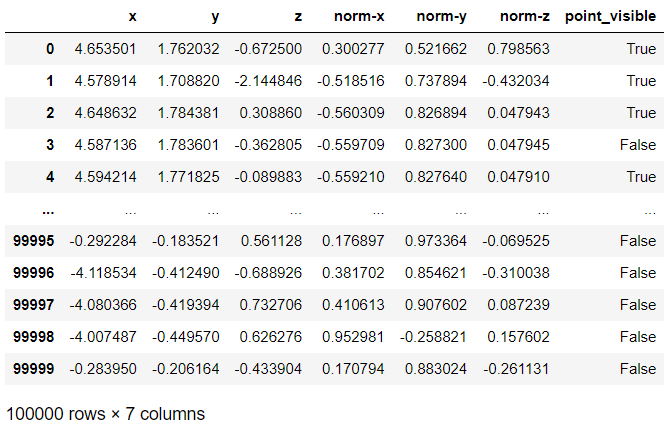
So, in order to convert the point cloud to a dataframe, each point in the point cloud can be represented in a single row by the following seven attribute columns:

1. X coordinate (float)
2. Y coordinate (float)
3. Z coordinate (float)
4. Normal vector coordinate in X direction (float)
5. Normal vector coordinate in Y direction (float)
6. Normal vector coordinate in Z direction (float)
7. Point visible (boolean True or False)

The point cloud can be converted to a dataframe by running the following lines of code:

# Creating a dataframe for the point cloud with the X, Y & Z positional coordinates
# and the normal unit vector coordinates in the X, Y & Z directions of all points.
pcd_df = pd.DataFrame(np.concatenate((np.asarray(pcd.points), np.asarray(pcd.normals)), axis=1),
                      columns=["x", "y", "z", "norm-x", "norm-y", "norm-z"]
                     )

# Adding a column to indicate whether the point is visible or not using the aggregated
# list of indexes of points from the hidden point removal operation above.
pcd_df["point_visible"] = False
pcd_df.loc[pt_map_aggregated, "point_visible"] = True

This would return a dataframe as shown below, where each point is a row represented by the seven attribute columns explained above.

Saving the point cloud and dataframe

The point clouds (before and after hidden point removal) and the dataframe can now be saved by running the following lines of code:

# Saving the entire point cloud as a .pcd file.
pcd_save_path = "data/3d_model.pcd"
o3d.io.write_point_cloud(pcd_save_path, pcd)

# Saving the point cloud with the hidden points removed as a .pcd file.
pcd_visible_save_path = "data/3d_model_hpr.pcd"
o3d.io.write_point_cloud(pcd_visible_save_path, pcd_visible)

# Saving the point cloud dataframe as a .csv file.
pcd_df_save_path = "data/3d_model.csv"
pcd_df.to_csv(pcd_df_save_path, index=False)