论文信息
论文标题:Pairwise Adversarial Training for Unsupervised Class-imbalanced Domain Adaptation
论文作者:Weili Shi, Ronghang Zhu, Sheng Li
论文来源:KDD 2022
论文地址:download
论文代码:download
视屏讲解:click
1 摘要
提出问题:类不平衡问题;
解决方法:
-
- 提出了一种新颖的成对对抗训练方法,该方法从源域和目标域的成对样本中生成对抗样本,并进一步利用这些样本来增强训练数据;
- 提出了一种新的优化算法来解决成对对抗训练问题;
2 问题定义
In class-imbalanced domain adaptation, both the source and target domains suffer from label distribution shift. We are given a source domain $\mathcal{D}_{s}=\left\{\left(x_{i}^{s}, y_{i}^{s}\right)\right\}_{i=1}^{N_{s}}$ with $N^{s}$ labelled samples and a target domain $\mathcal{D}_{t}=\left\{x_{i}^{t}\right\}_{i=1}^{N_{t}}$ with $N^{t}$ unlabelled samples. Each domain contains $K$ classes, and the class label is denoted as $y^{S} \in\{1,2, \ldots, K\}$ . Let $p$ and $q$ denote the probability distributions of the source and target domains, respectively. We assume that both the covariate shift (i.e., $p(x) \neq q(x)$ ) and label distribution shift (i.e., $p(y) \neq q(y)$ and $p(x \mid y) \neq q(x \mid y)$) exist in two domains. The model typically consists of a feature extractor $g: \mathcal{X} \rightarrow \mathcal{Z}$ and a classifier $f: \mathcal{Z} \rightarrow \boldsymbol{y}$ . The predicted label $\hat{y}=f(g(x))$ and empirical risk is defined as $\epsilon=\operatorname{Pr}_{x \sim \mathcal{D}}(\hat{y} \neq y)$ , where $y$ is ground-truth label. The source error and target error are denoted as $\epsilon_{S}$ and $\epsilon_{T}$ , respectively. Our goal is to train a model that can reduce gap between source and target domains and minimize $\epsilon_{S}$ and $\epsilon_{T}$ under label distribution shift.
3 方法
3.1 标签偏移
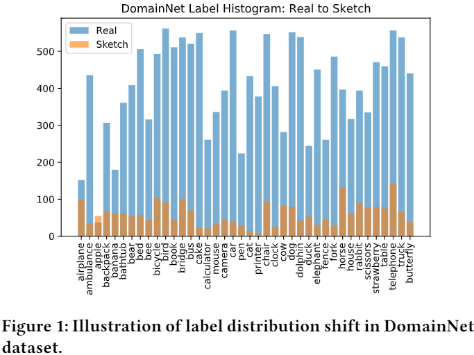
Note:简单增加两个域的数据来解决标签偏移是微不足道的,因为还要考虑域偏移的影响,本文通过生成对抗样本来缓解源域和目标域中的不平衡问题;
3.2 整体框架
整体框架:
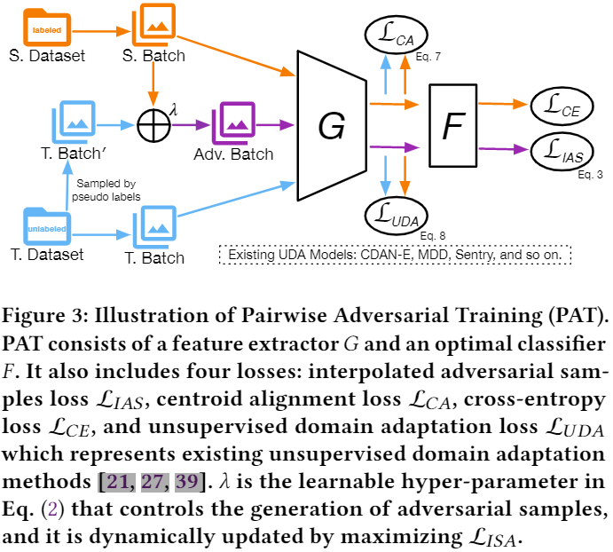
使用对抗训练增强模型鲁棒性,对抗损失如下:
$\begin{array}{l}\mathcal{L}_{c e}\left(x+\delta^{*}, y ; \theta\right) \\where \quad \delta^{*}:=\arg \max \mathcal{L}_{c e}(x+\delta, y ; \theta) , \|\delta\|_{p} \leq \epsilon \end{array} \quad\quad\quad(1)$
传统对抗训练在 CDA 中不适用的原因:
-
- 大多仅从原始样本的邻域生成对抗样本,没有考虑源域和目标域之间的域差距;
- 无法处理类不平衡问题;
基于上述两个原因,本文提出从源和目标域使用动态线性差值动态生成对抗样本来缓解类不平衡问题,以及 通过显式对齐源域和目标域的条件特征分布来减少域差异,如 Figure 3 所示:
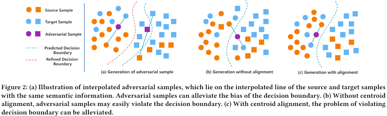
3.3 内插对抗样本生成
如 Figure2(a) 所示,对来自同一类的成对源和目标样本进行线性插值来生成对抗样本,插值对抗样本 (IAS) 应与其对应的源样本和目标样本具有相同的语义。通过动态利用内插对抗样本明确解决了源域中的数据不平衡问题,提高了无偏模型的泛化能力,并且可以隐式地解决目标域中的数据不平衡问题。
对于第 $k$ 类,插值的对抗样本可以定义为:
$X_{k}^{a d v}=\left\{x_{i}^{a d v} \mid x_{i}^{a d v}=x_{i}^{s}+\lambda\left(x_{i}^{t}-x_{i}^{s}\right), \lambda \in[0,1)^{C}, y_{i}^{s}=\hat{y}_{i}^{t}=k\right\} \quad\quad\quad(2)$
其中:
$\hat{y}_{i}^{t}$ 是通过分类器生成的伪标签;
尽管采用伪标签来生成对抗样本,但 PAT 对潜在的错误累积问题具有鲁棒性,原因:
-
- 错误分类的目标样本通常存在于决策边界,尽管目标样本的伪标签实际上并不正确,但由于新样本可能更接近源样本,因此生成的对抗样本很有可能仍然与相应的源样本保持相同的语义信息;
- 生成的对抗样本是动态产生的,随着模型逐渐收敛,不良对抗样本的不利影响可能减小;
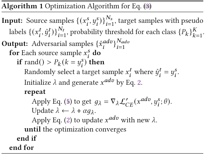
Note:本文中并非所有类都有相同的机会生成对抗样本,采用概率阈值 $P_{k}$ 来控制来自第 $k$ 类的一对源样本和目标样本的对抗样本的生成。
插值对抗样本的生成可以通过解决以下优化问题来实现:
$\begin{array}{l}\mathcal{L}_{I A S}:=\mathcal{L}_{C E}\left(\hat{x}^{a d v}, y ; \theta\right) \\\text { where } \quad \hat{x}^{a d v}=\underset{x^{a d v} \in \mathcal{X}^{a d v}}{\arg \max } \mathcal{L}_{C E}^{\prime}\left(x^{a d v}, y ; \theta\right)\end{array} \quad\quad\quad(3) $
外部最小化使用标准交叉熵损失 $\mathcal{L}_{C E}$,即:
$\mathcal{L}_{C E}\left(\hat{x}^{a d v}, y ; \theta\right)=-\log \left(\sigma_{y}\left(f\left(g\left(\hat{x}^{a d v}\right)\right)\right)\right) \quad\quad\quad(4)$
内部最大化使用交叉熵的修改版,可以缓解熵损失最大化时梯度爆炸或消失的问题,它写成:
$\mathcal{L}_{C E}^{\prime}\left(x^{a d v}, y ; \theta\right)=\log \left(1-\sigma_{y}\left(f\left(g\left(x^{a d v}\right)\right)\right)\right. \quad\quad\quad(5)$
本文生成对抗样本的方法如 Algorithm 1:
IAS 代码:


def get_perturb_point(self,input_source,labels_source):
    self.model.train(False)
    src_point = []
    tgt_point = []
    point_label = []

    for src_index,label in enumerate(labels_source):
        if torch.rand(1) > self.thresh_prob_class[label.cpu().item()]:
            cond_one = self.target_label == label
            cond_two = self.target_prob > self.thresh_prob_pesudo
            cond = torch.bitwise_and(cond_one, cond_two)
            cond_index = torch.nonzero(cond,as_tuple=True)[0]
            if cond_index.size(0) > 0:
                src_sample = input_source[src_index]
                tgt_index = cond_index[torch.randint(cond_index.size(0),(1,))]
                _,tgt_sample,_ = self.target_dataset[tgt_index]
                src_point.append(src_sample)
                tgt_point.append(tgt_sample)
                point_label.append(label)

    if len(point_label) <= 1:
        return None

    src_point = torch.stack(src_point)
    tgt_point = torch.stack(tgt_point)
    point_label = torch.as_tensor(point_label).long()

    src_point = src_point.to(self.device)
    tgt_point = tgt_point.to(self.device)
    point_label = point_label.to(self.device)

    perturb_num = src_point.size(0)
    cof = torch.rand(perturb_num,3,1,1,device=self.device)
    cof.requires_grad_(True)

    optim = SGD([cof],lr=0.001,momentum=0.9)
    loop = self.max_loop
    for i in range(loop):
        optim.zero_grad()
        perturbed_point = src_point + cof * (tgt_point - src_point)
        _,perturbed_output,_,_ = self.model(perturbed_point)

        perturbed_output_softmax = 1 - F.softmax(perturbed_output, dim=1)
        perturbed_output_logsoftmax = torch.log(perturbed_output_softmax.clamp(min=self.epsilon))
        loss = F.nll_loss(perturbed_output_logsoftmax, point_label,reduction='none')
        final_loss = torch.sum(loss)
        final_loss.backward()

        optim.step()
        cof.data.clamp_(0,1)
        self.model.zero_grad()

    cof = cof.detach()
    perturbed_point = src_point + cof * (tgt_point - src_point)
    self.model.train(True)
    return (perturbed_point,point_label)
3.4 类不平衡语义质心对齐
本文中并非所有类都有相同的机会生成对抗样本,采用概率阈值 $P_{k}$ 来控制来自第 $k$ 类的一对源样本和目标样本的对抗样本的生成。
${\large P_{k}=\frac{n_{k}}{n_{\max }+\tau}} \quad\quad\quad(6)$
其中:
$n_{k}$ 是第 $k$ 类的样本数;
$n_{\max }= \max _{k}\left\{n_{k}\right\}_{k=1}^{K}$;
此外,使用移动平均质心对齐[38],显式匹配两个域的质心来对齐源域和目标域的条件特征分布。
如 Figure 2b 所示,如果没有质心对齐,则可能会从一对样本中生成对抗性样本,其中一个样本与其他类未对齐,从而使对抗性样本的嵌入超出决策边界。 通过 Figure 2c 所示的质心对齐,可以消除这种越界对抗样本的出现。 移动平均质心对齐的损失函数定义为:
$\mathcal{L}_{C A}=\sum_{k=1}^{K} \operatorname{dist}\left(C_{k}^{S}, C_{k}^{t}\right) \quad\quad\quad(7)$
其中,$C_{k}^{s}$ 和 $C_{k}^{t}$ 分别表示源域和目标域中第 $k$ 类的质心。
3.5 用于类不平衡域自适应的 PAT
训练目标:
$\mathcal{L}=\mathcal{L}_{U D A}+\mathcal{L}_{C E}+\alpha \mathcal{L}_{I A S}+\beta \mathcal{L}_{C A} \quad\quad\quad(8)$
其中:
-
- interpolated adversarial samples loss $\mathcal{L}_{I A S}$ which aims to dynamically generate adversarial samples to alleviate imbalance issue
- centroid alignment loss $\mathcal{L}_{C A}$ is designed to align the conditional feature distributions of source and target
- standard cross-entropy loss $\mathcal{L}_{C E}$
- unsupervised domain adaptation loss $\mathcal{L}_{U D A}$ which is adopted from existing UDA methods
4 实验
略
5 总结
略
- Class-imbalanced Unsupervised Adversarial Adaptation imbalancedclass-imbalanced unsupervised adversarial adaptation class-imbalanced class-imbalanced classification re-balancing domain unsupervised adversarial contrastive tri-training unsupervised asymmetric adaptation adaptation domain moka adversarial unsupervised intra-class adaptation similarity mensa unsupervised adaptation ensemble domain discriminative unsupervised adaptation backpropagation unsupervised adaptation domain