Precomputed Radiance Transfer(games202)
关于BRDF可以看看这篇文章基于物理着色:BRDF
物体在不同光照下的表现不同,PRT(Precomputed Radiance Transfer) 是一个计算物体在不同光照下表现的方法。光线在一个环境中,会经历反射,折射,散射,甚至还会物体的内部进行散射。为了模拟具有真实感的渲染结果,传统的Path Tracing 方法需要考虑来自各个方向的光线、所有可能的传播形式并且收敛速度极慢。PRT 通过一种预计算方法,该方法在离线渲染的 Path Tracing 工具链中预计算 lighting 以及 light transport 并将它们用球谐函数拟合后储存,这样就将时间开销转移到了离线中。最后通过使用这些预计算好的数据,我们可以轻松达到实时渲染严苛的时间要求,同时渲染结果可以呈现出全局光照的效果。
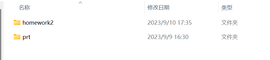
作业2的文件夹里有两个子文件夹homework2是和作业一类似的代码框架,prt文件夹则是我们需要用来预计算的c++代码。
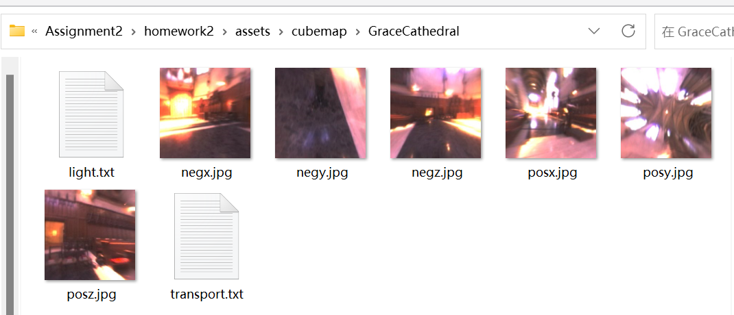
我们首先需要完成 prt\src\prt.cpp文件的预计算的代码部分,然后编译完成项目后,运行 \prt\build\Debug\nori.exe文件,参数指定为prt.xml文件。该文件可以修改内容来生产不同环境(indoor,skybox,Connell box以及GraceCathedral)的光照项的球谐系数以及传输项的球谐系数。生产的预计算文件必须要放在 homework2\assets\cubemap下对应的环境贴图文件夹下才能生效。
球谐函数(Spherical Harmonics,SH)
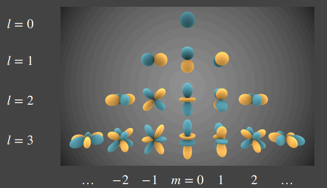
个人理解的球谐函数就类似泰勒展开一样,对于一个任意的函数 \(y(x)\),我们可以用泰勒展开\(y(x)=c_0+c_1x+c_2x^2+...+c_nx^n\),那么只要我们知道\(c_0, c_1, c_2 ..., c_n\),我们就能够还原出\(y(x)\)。这里的\(x, x^2, x^3...x^n\)也就是我们能够确定的基函数,我们需要求出来的就是系数\(c_0, c_1, c_2 ..., c_n\)。那么在三维空间中也是同样的道理,球谐系数SH就是类似于\(x^1,...x^n\)的基函数,但是远远复杂的多。球谐函数如图所示。
如果我们能求出每一个基函数前面的系数,我们也能像泰勒展开一样还原出原函数。那么要如何求出系数呢?由于球谐函数的正交性
只要我们让一个基函数和原函数做积分,那么得到的结果就会是该基函数的系数。
这里的\(c_i\)只是一个数而已。在PRT中,要把光照和传输项分开求系数。
再用黎曼积分求解原方程
由于SH的正交性,最终结果变成了
我们会惊奇的发现,复杂的函数积分变成了简单的数值相乘。如果不用球谐函数简化计算,考虑对原始的渲染方程做黎曼积分的开销。
这里有\(i,o,n\)三个参数再考虑到\(RGB\)三个通道,如果在64*64的分辨率下,至少需要的开销就是\(6*64*64\)。通过球谐函数(这里考虑三阶9个基函数以及RGB三个通道)后仅仅需要\(9 * 3\),最终输出的是一个三维的(RGB)颜色向量。
关于球谐函数可以参考球谐函数介绍(Spherical Harmonics)以及球谐光照——球谐函数。
综上可知,我只需要分别的预计算出光照项的球谐系数以及每个顶点的传输项的球谐系数。
光照项的预计算
直接根据公式来计算
//prt.cpp
template <size_t SHOrder>
std::vector<Eigen::Array3f> PrecomputeCubemapSH(const std::vector<std::unique_ptr<float[]>> &images,
                                                const int &width, const int &height,
                                                const int &channel)
{
    ...

    constexpr int SHNum = (SHOrder + 1) * (SHOrder + 1); //n阶SH共有n^2个系数
    std::vector<Eigen::Array3f> SHCoeffiecents(SHNum);
    for (int i = 0; i < SHNum; i++)
        SHCoeffiecents[i] = Eigen::Array3f(0);
    float sumWeight = 0;
    for (int i = 0; i < 6; i++)
    {
        for (int y = 0; y < height; y++)
        {
            for (int x = 0; x < width; x++)
            {
                // TODO: here you need to compute light sh of each face of cubemap of each pixel
                // TODO: 此处你需要计算每个像素下cubemap某个面的球谐系数
                Eigen::Vector3f dir = cubemapDirs[i * width * height + y * width + x];
                int index = (y * width + x) * channel;
                Eigen::Array3f Le(images[i][index + 0], images[i][index + 1],
                                    images[i][index + 2]);//images是按照RGBRGBRGB排列

                auto delta_wi = CalcArea(x, y, height, width);
                Eigen::Vector3d _dir(Eigen::Vector3d(dir[0], dir[1], dir[2]).normalized());//这里dir要变成Eigen::Vector3d类型
                for(int l=0; l<=SHOrder; l++)
                {
                    for(int m=-l; m<=l; m++)
                    {
                        SHCoeffiecents[sh::GetIndex(l, m)] += Le * sh::EvalSH(l, m, _dir) * delta_wi;
                    }
                }
            }
        }
    }
    return SHCoeffiecents;
}
三层 for循环遍历了6个面上每个像素,光照项系数是所有的这些点共同作用的结果。
这边的 index 的取值是考虑了RGB,从前面的函数 LoadCubemapImages 中可以看到 float*image = stbi_loadf(filename.c_str(),&w,&h,&c,3);这里image返回的结果是RGBRGBRGBRGB格式排列,这也就是为什么 index 还要乘以一个channel值,并且取得贴图的RGB值需要的就是连续的三个值 Le(images[i][index + 0], images[i][index + 1], images[i][index + 2]);。
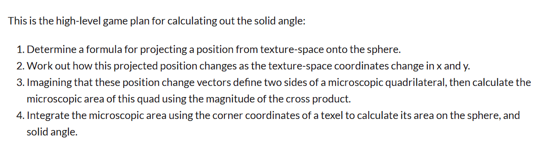
delta_wi的计算通过函数 CalcArea,这个函数做的就是如下步骤,具体数学原理参考CUBEMAP TEXEL SOLID ANGLE
球谐函数的\(l,m\)的关系如下图
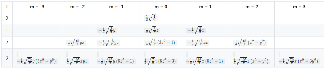
可以看到前三阶共有9个基函数,根据\(l,m\)通过函数 sh::EvalSH()得到对应的基函数。需要注意第三个参数是方向向量,需要类型是 Eigen::Vector3d而不是 Eigen::Vector3d。
传输项的预计算
Diffuse Unshadowed
在这种Diffuse Unshadowed下,渲染方程简化成了
光照传输项就变成了
//prt.cpp
for (int i = 0; i < mesh->getVertexCount(); i++)
        {
            const Point3f &v = mesh->getVertexPositions().col(i);
            const Normal3f &n = mesh->getVertexNormals().col(i);
            auto shFunc = [&](double phi, double theta) -> double {
                Eigen::Array3d d = sh::ToVector(phi, theta);
                const auto wi = Vector3f(d.x(), d.y(), d.z());
                double H = wi.dot(n);
                if (m_Type == Type::Unshadowed)
                {
                    // TODO: here you need to calculate unshadowed transport term of a given direction
                    // TODO: 此处你需要计算给定方向下的unshadowed传输项球谐函数值
                    return H > 0.0? H : 0;
                }
                else
                {
                }
            };
            auto shCoeff = sh::ProjectFunction(SHOrder, shFunc, m_SampleCount);
            for (int j = 0; j < shCoeff->size(); j++)
            {
                m_TransportSHCoeffs.col(i).coeffRef(j) = (*shCoeff)[j];
            }
        }
和光照项不同,光照项系数只有一组*3(RGB),传输项系数是每个顶点都有一组。这里通过 sh::ProjectFunction来进行计算球谐函数系数,还有一个不同之处在于,这个函数计算的方法和计算光照项不同,它是在球面上均匀采样并用蒙特卡洛积分法来计算的。应用蒙特卡罗积分,通过投影操作获得的系数可以使用n个样本进行近似。每一个方向\(\omega_i\)采样是\(max(n\cdot \omega_i,0)\),光照与传输函数采样方向集合为\(\omega_i\),\(1<i<n\)
由于这些函数是在所有可能方向的空间上定义的(几何上,该空间可视为单位球体的表面),因此在该表面上出现任何样本(方向)的概率将是 1/该单位球体面积 (\(\frac{1}{4\pi}\)),故${p(\omega_i)} =\frac{1}{4\pi} $
//spherical_harmonics.cc
std::unique_ptr<std::vector<double>> ProjectFunction(
    int order, const SphericalFunction& func, int sample_count) {
  CHECK(order >= 0, "Order must be at least zero.");
  CHECK(sample_count > 0, "Sample count must be at least one.");

  // This is the approach demonstrated in [1] and is useful for arbitrary
  // functions on the sphere that are represented analytically.
  const int sample_side = static_cast<int>(floor(sqrt(sample_count)));
  std::unique_ptr<std::vector<double>> coeffs(new std::vector<double>());
  coeffs->assign(GetCoefficientCount(order), 0.0);

  // generate sample_side^2 uniformly and stratified samples over the sphere
  std::random_device rd;
  std::mt19937 gen(rd());
  std::uniform_real_distribution<> rng(0.0, 1.0);
  for (int t = 0; t < sample_side; t++) {
    for (int p = 0; p < sample_side; p++) {
      double alpha = (t + rng(gen)) / sample_side;
      double beta = (p + rng(gen)) / sample_side;
      // See http://www.bogotobogo.com/Algorithms/uniform_distribution_sphere.php
      double phi = 2.0 * M_PI * beta;
      double theta = acos(2.0 * alpha - 1.0);

      // evaluate the analytic function for the current spherical coords
      double func_value = func(phi, theta);

      // evaluate the SH basis functions up to band O, scale them by the
      // function's value and accumulate them over all generated samples
      for (int l = 0; l <= order; l++) {
        for (int m = -l; m <= l; m++) {
          double sh = EvalSH(l, m, phi, theta);
          (*coeffs)[GetIndex(l, m)] += func_value * sh;
        }
      }
    }
  }

  // scale by the probability of a particular sample, which is
  // 4pi/sample_side^2. 4pi for the surface area of a unit sphere, and
  // 1/sample_side^2 for the number of samples drawn uniformly.
  double weight = 4.0 * M_PI / (sample_side * sample_side);
  for (unsigned int i = 0; i < coeffs->size(); i++) {
     (*coeffs)[i] *= weight;
  }

  return coeffs;
}
没有理解为什么光照项不采用蒙特卡洛积分,或者为什么传输项用和光照项一样的计算方法?
Diffuse Shadowed
和Unshadowed基本上差不都,多了一个\(V(\omega_i)\)项,只需要增加光线传播是否被物体遮挡的判断条件即可
//prt.cpp
for (int i = 0; i < mesh->getVertexCount(); i++)
        {
            const Point3f &v = mesh->getVertexPositions().col(i);
            const Normal3f &n = mesh->getVertexNormals().col(i);
            auto shFunc = [&](double phi, double theta) -> double {
                Eigen::Array3d d = sh::ToVector(phi, theta);
                const auto wi = Vector3f(d.x(), d.y(), d.z());
                double H = wi.dot(n);
                if (m_Type == Type::Unshadowed)
                {
                    // TODO: here you need to calculate unshadowed transport term of a given direction
                    // TODO: 此处你需要计算给定方向下的unshadowed传输项球谐函数值
                    return H > 0.0? H : 0;
                }
                else
                {
		    // TODO: here you need to calculate shadowed transport term of a given direction
                    // TODO: 此处你需要计算给定方向下的shadowed传输项球谐函数值
                    if(H > 0.0 && !scene->rayIntersect(Ray3f(v, wi.normalized())))
                        return H;
                    return 0;
                }
            };
            auto shCoeff = sh::ProjectFunction(SHOrder, shFunc, m_SampleCount);
            for (int j = 0; j < shCoeff->size(); j++)
            {
                m_TransportSHCoeffs.col(i).coeffRef(j) = (*shCoeff)[j];
            }
        }
Diffuse Inter-reflection(bonus)
按照上面的步骤,模仿 ProjectFunction()函数采样蒙特卡洛积分。这个函数类似于光线追踪,将光线进行递归的传播。
//prt.cpp
std::unique_ptr<std::vector<double>> computeInterreflectionSH(Eigen::MatrixXf* directTSHCoeffs, const Point3f& pos, const Normal3f& normal, const Scene* scene, int bounces)
{
    std::unique_ptr<std::vector<double>> coeffs(new std::vector<double>());
    coeffs->assign(SHCoeffLength, 0.0);

    if (bounces > m_Bounce)
        return coeffs;

    const int sample_side = static_cast<int>(floor(sqrt(m_SampleCount)));
    std::random_device rd;
    std::mt19937 gen(rd());
    std::uniform_real_distribution<> rng(0.0, 1.0);
    for (int t = 0; t < sample_side; t++) {
        for (int p = 0; p < sample_side; p++) {
            double alpha = (t + rng(gen)) / sample_side;
            double beta = (p + rng(gen)) / sample_side;
            double phi = 2.0 * M_PI * beta;
            double theta = acos(2.0 * alpha - 1.0);
	    //这边模仿ProjectFunction函数写

            Eigen::Array3d d = sh::ToVector(phi, theta);
            const auto wi = Vector3f(d.x(), d.y(), d.z());
            double H = wi.normalized().dot(normal);
            Intersection its;
            if (H > 0.0 && scene->rayIntersect(Ray3f(pos, wi.normalized()), its))
            {
                MatrixXf normals = its.mesh->getVertexNormals();
                Point3f idx = its.tri_index;
                Point3f hitPos = its.p;
                Vector3f bary = its.bary;

                Normal3f hitNormal =
                    Normal3f(normals.col(idx.x()).normalized() * bary.x() +
                        normals.col(idx.y()).normalized() * bary.y() +
                        normals.col(idx.z()).normalized() * bary.z())
                    .normalized();

                auto nextBouncesCoeffs = computeInterreflectionSH(directTSHCoeffs, hitPos, hitNormal, scene, bounces + 1);

                for (int i = 0; i < SHCoeffLength; i++)
                {
                    auto interpolateSH = (directTSHCoeffs->col(idx.x()).coeffRef(i) * bary.x() +
                        directTSHCoeffs->col(idx.y()).coeffRef(i) * bary.y() +
                        directTSHCoeffs->col(idx.z()).coeffRef(i) * bary.z());

                    (*coeffs)[i] += (interpolateSH + (*nextBouncesCoeffs)[i]) * H;
                }
            }
        }
    }

    for (unsigned int i = 0; i < coeffs->size(); i++) {
        (*coeffs)[i] /= sample_side * sample_side;
    }

    return coeffs;
}
然后补充 preprocess函数
if (m_Type == Type::Interreflection)
        {
            // TODO: leave for bonus
            for (int i = 0; i < mesh->getVertexCount(); i++)
            {
                const Point3f& v = mesh->getVertexPositions().col(i);
                const Normal3f& n = mesh->getVertexNormals().col(i).normalized();
                auto indirectCoeffs = computeInterreflectionSH(&m_TransportSHCoeffs, v, n, scene, 1);
                for (int j = 0; j < SHCoeffLength; j++)
                {
                    m_TransportSHCoeffs.col(i).coeffRef(j) += (*indirectCoeffs)[j];
                }
                std::cout << "computing interreflection light sh coeffs, current vertex idx: " << i << " total vertex idx: " << mesh->getVertexCount() << std::endl;
            }
        }
球谐光照的实时计算
我们已经完成了 prt文件夹中预计算的部分,接下来完成 homework2中实时计算。
在 materials文件夹下创建文件 PRTMaterial.js,代码如下
class PRTMaterial extends Material {

    constructor(vertexShader, fragmentShader) {

        super({
            'uPrecomputeL[0]': { type: 'precomputeL', value: null}, //0,1,2 表示RGB
            'uPrecomputeL[1]': { type: 'precomputeL', value: null},
            'uPrecomputeL[2]': { type: 'precomputeL', value: null},
        },
        ['aPrecomputeLT'],
        vertexShader, fragmentShader, null);
    }
}

async function buildPRTMaterial(vertexPath, fragmentPath) {


    let vertexShader = await getShaderString(vertexPath);
    let fragmentShader = await getShaderString(fragmentPath);

    return new PRTMaterial(vertexShader, fragmentShader);

}
这里的 uPrecomputeL[0], uPrecomputeL[1], uPrecomputeL[2]分别是光照项RGB的预计算球谐系数。
然后在 loadOBJ.js里面创建这个材质
switch (objMaterial) {
	case 'PhongMaterial':
		material = buildPhongMaterial(colorMap, mat.specular.toArray(), light, Translation, Scale, "./src/shaders/phongShader/phongVertex.glsl", "./src/shaders/phongShader/phongFragment.glsl");
		shadowMaterial = buildShadowMaterial(light, Translation, Scale, "./src/shaders/shadowShader/shadowVertex.glsl", "./src/shaders/shadowShader/shadowFragment.glsl");
		break;
	// TODO: Add your PRTmaterial here

	//Edit Start
	case 'PRTMaterial':
		material = buildPRTMaterial("./src/shaders/prtShader/prtVertex.glsl", "./src/shaders/prtShader/prtFragment.glsl");
		break;
	//Edit End

	case 'SkyBoxMaterial':
		material = buildSkyBoxMaterial("./src/shaders/skyBoxShader/SkyBoxVertex.glsl", "./src/shaders/skyBoxShader/SkyBoxFragment.glsl");
		break;
}
预计算的光照系数和传输系数保存咋txt文件里面,在 engine.js里面把数据储存在了两个全局变量 precomputeL、precomputeLT 中。其中 precomputeL 将预计算环境光的 SH vector 保存为一个三维 Array,第一个维度表示属于哪组 cubemap 贴图,第二个维度表示 SH 系数,第三个维度表示 RGB;precomputeLT 将预计算 light transfer 的 SH vector保存为一个二维 Array,第一个维度表示属于哪组 cubemap 贴图,第二个维度是长度为 V ertexCount ∗ SHCoeff icientCount 的数组,这样可以方便后续绑定到attribute mat3 类型的变量中。
在 WebGlRenderer.js中将 precomputeL传给Shader
for (let k in this.meshes[i].material.uniforms) {

    ...

    let Mat3Value = getMat3ValueFromRGB(precomputeL[guiParams.envmapId])
    for(let j = 0; j < 3; j++){
        if (k == 'uPrecomputeL['+j+']') { //+来连接' '
            gl.uniformMatrix3fv(
                this.meshes[i].shader.program.uniforms[k],
                false,
                Mat3Value[j]);
        }
    }
}
这里根据实际的场景贴图cubemap选择对应的SH系数,通过 getMat3ValueFromRGB函数来分开RGB
function getMat3ValueFromRGB(precomputeL){

    let colorMat3 = [];
    for(var i = 0; i<3; i++){
        colorMat3[i] = mat3.fromValues( precomputeL[0][i], precomputeL[1][i], precomputeL[2][i],
					precomputeL[3][i], precomputeL[4][i], precomputeL[5][i],
					precomputeL[6][i], precomputeL[7][i], precomputeL[8][i] );
	}
    return colorMat3;
}
RGB对应的SH系数被分成3*3的矩阵
precomputeLT是在 MeshRender.js里完成的,这一部分作业框架已经帮我们完成了。由于每个顶点都有自己的传输项球谐系数,所以要把它绑定成顶点属性。这里似乎每一个顶点属性都会创建一个buffer,之前学OpenGL的时候,顶点属性共用一个buffer的,不懂其中区别。
在shader里面 aPrecomputeLT是33的mat3,似乎要给mat3的类型需要绑定三次vec3,所以代码就是如下结构。gl.vertexAttribPointer的每个参数的含义可以看这篇文章WebGLRenderingContext.vertexAttribPointer(),阅读 shader.js可以知道第一个参数实际上通过 gl.getAttribLocation()函数得到的显卡提供的 aPrecomputeLT的索引,我们可以使用显卡提供的索引,而不是自己设置索引,这样可以避免重新链接着色器程序。*
draw(camera) {

	...

	// Bind attribute mat3 - LT
	const buf = gl.createBuffer();
	gl.bindBuffer(gl.ARRAY_BUFFER, buf);
	gl.bufferData(gl.ARRAY_BUFFER, new Float32Array(precomputeLT[guiParams.envmapId]), gl.STATIC_DRAW);

	for (var ii = 0; ii < 3; ++ii) {
		gl.enableVertexAttribArray(this.shader.program.attribs['aPrecomputeLT'] + ii);
		gl.vertexAttribPointer(this.shader.program.attribs['aPrecomputeLT'] + ii, 3, gl.FLOAT, false, 36, ii * 12);
	}

	...
}
最后需要完成shader的代码,这里就是完成\(L(o) \approx \rho \sum l_i T_i\)的计算,循环是因为要计算RGB三个通道的值。
//prtVertex.glsl
attribute vec3 aVertexPosition;
attribute vec3 aNormalPosition;
attribute mat3 aPrecomputeLT;

uniform mat4 uModelMatrix;
uniform mat4 uViewMatrix;
uniform mat4 uProjectionMatrix;

uniform mat3 uPrecomputeL[3];

varying highp vec3 vNormal;
varying highp mat3 vPrecomputeLT;
varying highp vec3 vColor;

float L_dot_LT(mat3 PrecomputeL, mat3 PrecomputeLT) {
  vec3 L_0 = PrecomputeL[0];
  vec3 L_1 = PrecomputeL[1];
  vec3 L_2 = PrecomputeL[2];
  vec3 LT_0 = PrecomputeLT[0];
  vec3 LT_1 = PrecomputeLT[1];
  vec3 LT_2 = PrecomputeLT[2];
  return dot(L_0, LT_0) + dot(L_1, LT_1) + dot(L_2, LT_2);
}

void main(void) {
  // 无实际作用,避免aNormalPosition被优化后产生警告
  vNormal = (uModelMatrix * vec4(aNormalPosition, 0.0)).xyz;

  for(int i = 0; i < 3; i++)
  {
    vColor[i] = L_dot_LT(aPrecomputeLT, uPrecomputeL[i]);
  }

  gl_Position = uProjectionMatrix * uViewMatrix * uModelMatrix * vec4(aVertexPosition, 1.0);
}
//prtFragment.glsl

#ifdef GL_ES
precision mediump float;
#endif

varying highp vec3 vColor;

void main(){
  gl_FragColor = vec4(vColor, 1.0);
}
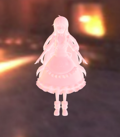
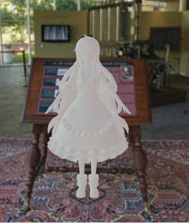
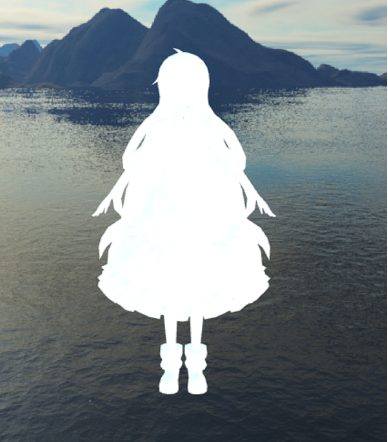
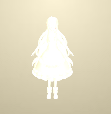
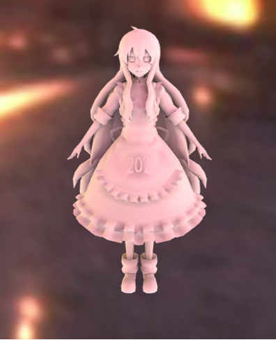
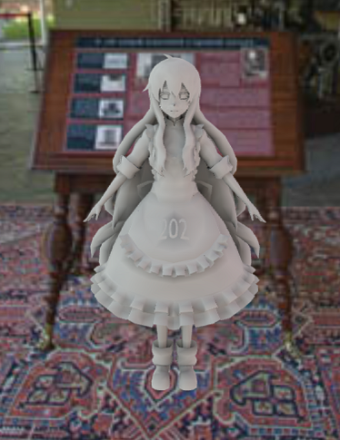
最终效果
要记住在cubemap的所有场景文件夹下都要放入计算出的 light.txt和 transport.txt文件,否在结果就是黑屏。
Diffuse Unshadowed
修改 ...\prt\scenes文件夹下面的 prt.xml文件,如下注释所示
<scene>
    ...

    <!-- Render the visible surface normals -->
    <integrator type="prt">
		<string name="type" value="unshadowed" />//修改成unshadowed
		<integer name="bounce" value="1" />
		<integer name="PRTSampleCount" value="100" />
		<string name="cubemap" value="cubemap/Indoor" />//indoor,skybox,GraceCathedral,cornellbox都要计算
	</integrator>

    ...
</scene>
Diffuse Shadowed
<scene>
    ...

    <!-- Render the visible surface normals -->
    <integrator type="prt">
		<string name="type" value="shadowed" />//修改成shadowed
		<integer name="bounce" value="1" />
		<integer name="PRTSampleCount" value="100" />
		<string name="cubemap" value="cubemap/Indoor" />//indoor,skybox,GraceCathedral,cornellbox都要计算
	</integrator>

    ...
</scene>
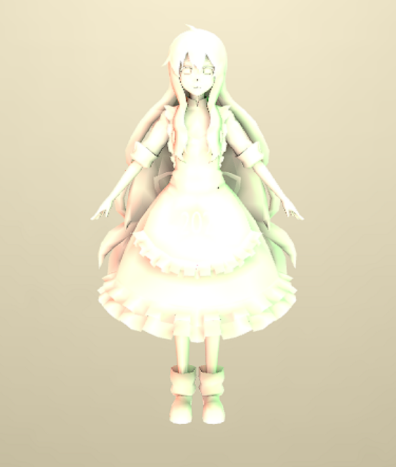
有明显的感觉到过亮了,这是因为作业给的代码框架没有把传输球谐系数除以\(\pi\),可以参考这篇文章进行修改GAMES202-作业2: Precomputed Radiance Transfer(球谐函数)
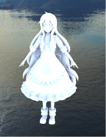
Diffuse Inter-reflection
<scene>
    ...

    <!-- Render the visible surface normals -->
    <integrator type="prt">
		<string name="type" value="interreflection" />//修改成interreflection
		<integer name="bounce" value="1" />
		<integer name="PRTSampleCount" value="100" />
		<string name="cubemap" value="cubemap/Indoor" />//indoor,skybox,GraceCathedral,cornellbox都要计算
	</integrator>

    ...
</scene>