VINS 中的旋转外参初始化
为了使这个两个传感器融合,我们首先需要做的事情是将两个传感器的数据对齐,除了时间上的对齐,还有空间上的对齐。空间上的对齐通俗的讲就是将一个传感器获取的数据统一到另一个传感器的坐标系中,其关键在于确定这两个传感器之前的外参,本文将详细介绍 VINS_Mono 中 camera-imu 的旋转外参标定算法原理并对其代码进行解读(VINS-Fusion中也是一样的)。
相机与 IMU 之间的相对旋转如下图所示:
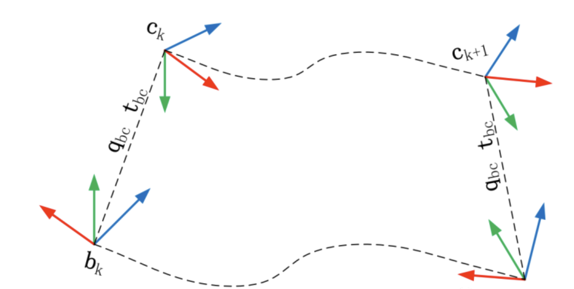
上图表示相机和 IMU 集成的系统从到的运动,其中视觉可以通过特征匹配求得到时刻的旋转增量,同时 IMU 也可以通过积分得到到时刻的旋转增量。两个求得的旋转增量应当是相同的,因此分别将在自己坐标系下求得的增量转移到对方的坐标系下,即经过 \(\mathbf{q}_{bc}\) 变换后应当还是相同的。
相邻两时刻 \(k\) , \(k + 1\) 之间有: IMU 旋转积分 \(\mathbf{q}_{b_{k} b_{k+1}}\) ,视觉测量 \(\mathbf{q}_{c_{k} c_{k+1}}\)。则有:
上面的式子可以写成:
其中 \(\left[ \dot{\ \ \ } \right]_L, \left[ \dot{\ \ \ } \right]_R\) 表示 left and right quaternion multiplication,不清楚可以看附录,其实就是四元数乘法换了个表达形式。
将多个时刻线性方程累计起来,并加上鲁棒核权重得到:
该线性方程为超定方程,有最小二乘解。采用 SVD 进行求解。
- 代码
bool InitialEXRotation::CalibrationExRotation(vector<pair<Vector3d, Vector3d>> corres, Quaterniond delta_q_imu, Matrix3d &calib_ric_result)
{
    frame_count++;
    Rc.push_back(solveRelativeR(corres));                               // 对极几何计算出的 R,t 约束
    Rimu.push_back(delta_q_imu.toRotationMatrix());     // IMU 预积分的得到的 R,t 约束
    Rc_g.push_back(ric.inverse() * delta_q_imu * ric);       // 将imu预积分转换到相机坐标系

    Eigen::MatrixXd A(frame_count * 4, 4);
    A.setZero();
    int sum_ok = 0;
    for (int i = 1; i <= frame_count; i++)
    {
        Quaterniond r1(Rc[i]);
        Quaterniond r2(Rc_g[i]);

        // A.angularDistance(B):是求两个旋转之间的角度差,用弧度表示
        double angular_distance = 180 / M_PI * r1.angularDistance(r2);
        ROS_DEBUG(
            "%d %f", i, angular_distance);

        double huber = angular_distance > 5.0 ? 5.0 / angular_distance : 1.0; // huber 核函数作加权
        ++sum_ok;
        // L R 分别为左乘和右乘矩阵
        Matrix4d L, R;

        double w = Quaterniond(Rc[i]).w();
        Vector3d q = Quaterniond(Rc[i]).vec();
        L.block<3, 3>(0, 0) = w * Matrix3d::Identity() + Utility::skewSymmetric(q);
        L.block<3, 1>(0, 3) = q;
        L.block<1, 3>(3, 0) = -q.transpose();
        L(3, 3) = w;

        Quaterniond R_ij(Rimu[i]);
        w = R_ij.w();
        q = R_ij.vec();
        R.block<3, 3>(0, 0) = w * Matrix3d::Identity() - Utility::skewSymmetric(q);
        R.block<3, 1>(0, 3) = q;
        R.block<1, 3>(3, 0) = -q.transpose();
        R(3, 3) = w;

        A.block<4, 4>((i - 1) * 4, 0) = huber * (L - R);
    }

    // svd 分解中最小奇异值对应的右奇异向量作为旋转四元数
    JacobiSVD<MatrixXd> svd(A, ComputeFullU | ComputeFullV);
    Matrix<double, 4, 1> x = svd.matrixV().col(3);
    Quaterniond estimated_R(x);
    // 所求的 x 是q^b_c,在最后需要转换成旋转矩阵并求逆。
    ric = estimated_R.toRotationMatrix().inverse();
    //cout << svd.singularValues().transpose() << endl;
    //cout << ric << endl;
    Vector3d ric_cov;
    ric_cov = svd.singularValues().tail<3>();
    // 至少迭代计算了WINDOW_SIZE次,且R的奇异值大于0.25才认为标定成功
    if (frame_count >= WINDOW_SIZE && ric_cov(1) > 0.25)
    {
        calib_ric_result = ric;
        return true;
    }
    else
        return false;
}
Appendix
- The product of two quaternions is bi-linear and can be expressed as two equivalent matrix products, namely
\(\quad\)where \([\mathbf{q}]_{L}\) and \([\mathbf{q}]_{R}\) are respectively the left- and right- quaternion-product matrices
\(\quad\)then